
Advanced Robotics / Reinforcement Learning · Lesson 07
Function Approximation Intuition
Est. 65–80 min
Why
Why this lesson matters
In Lesson 6 the table broke in two ways: it grew as bins^variables, and each box had to be learnt on its own. Function approximation fixes both. Instead of one stored number per (state, action), we keep a small set of weights w and compute Q(s, a; w) from the state. Change a weight and the estimate changes for a whole neighbourhood of states at once — that is generalisation.
Today you will see one update spread to nearby angles, beat the 36-, 180- and 900-bin tables on the same servo task with just 33 weights, learn how the choice of features decides what the robot can learn, and run a linear Q-learner on the light-seeker with 18 weights. This is the exact idea a DQN (Lesson 8) uses — with a neural network as the formula.
Concept
From boxes to a formula
1. Table vs function
| Q-table | Function approximation | |
|---|---|---|
| What is stored | one number per (state, action) | a fixed set of weights w |
| Size | grows as bins^variables × actions | chosen by you (tens to millions of weights) |
| Learning at 40° | changes only the 40° box | also changes 41°, 45°, 50°… (less and less with distance) |
| Unseen state | still at its starting value | gets a sensible guess from its neighbours |
| Risk | slow, but each box is exact | one update can also spoil a far-away guess |
2. Linear Q with features
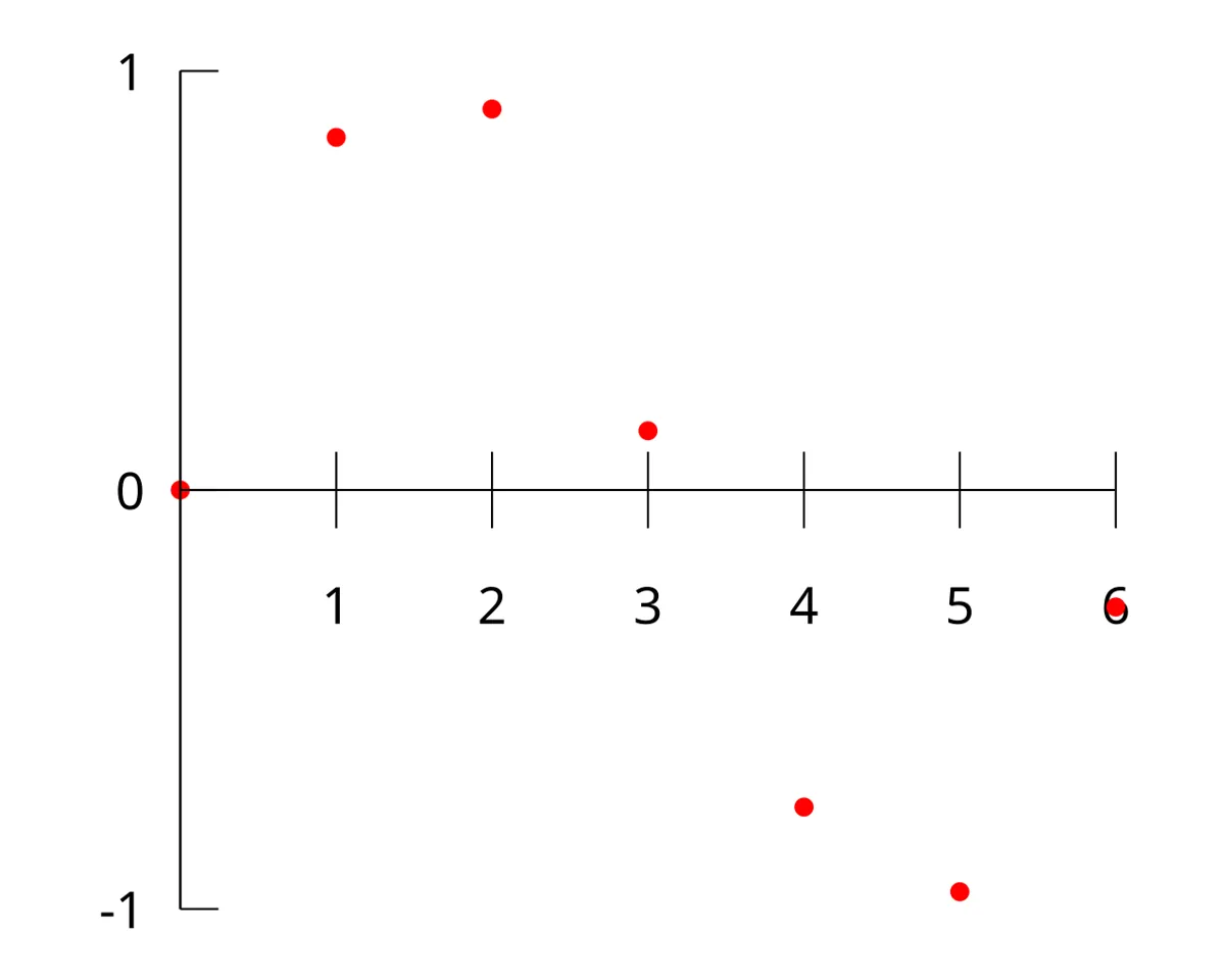
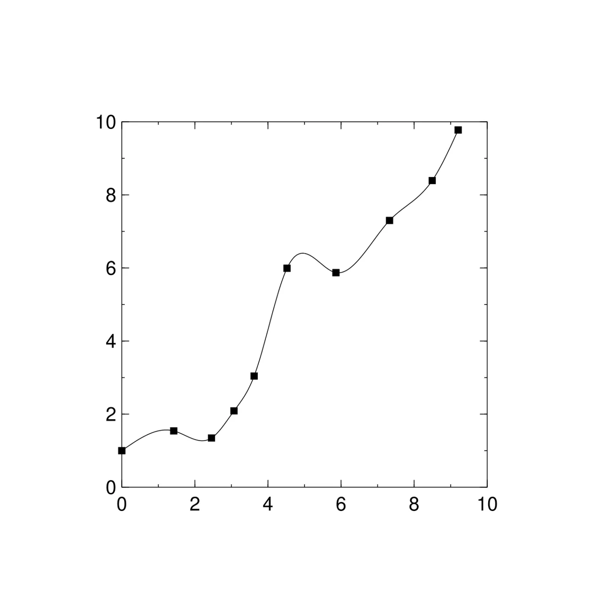
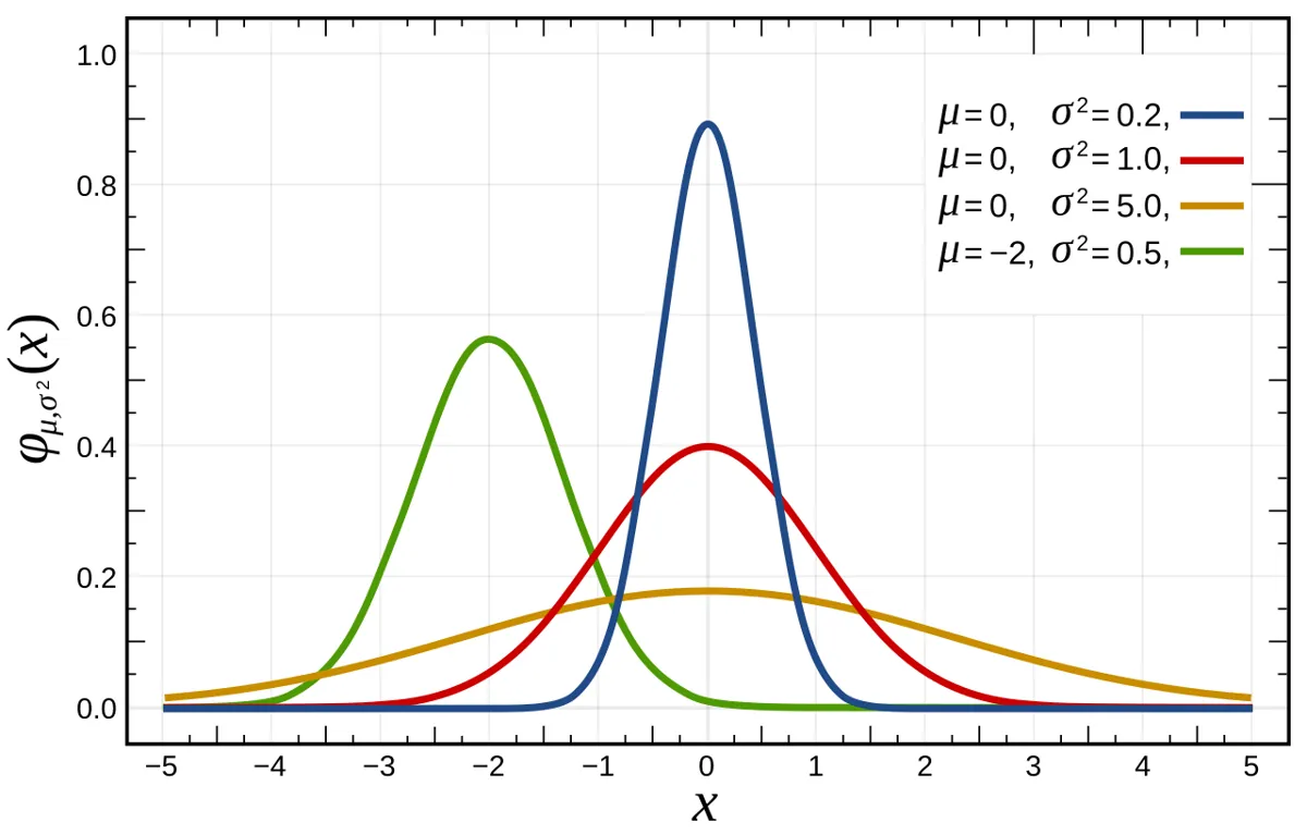
The simplest approximator is linear: turn the state into a list of features f(s) (numbers that describe it), and keep one weight per feature per action. Then Q(s, a) = w_a · f(s) = w_a,1·f₁(s) + w_a,2·f₂(s) + … For a servo angle, a good feature set is a few bumps (radial basis functions, RBFs): each bump is 1 when the angle is at its centre and fades to 0 further away. A radial basis function is a function whose value depends only on the distance from a fixed centre point.
def rbf_features(x, centres, width):
    return [math.exp(-((x - c) / width) ** 2) for c in centres] + [1.0]   # bumps + constant

# Q(x, a) = sum(W[a][i] * f[i])
err = r + 0.9 * max(Q(x2, b) for b in actions) - Q(x, a)     # same TD error as Q-learning
step = 0.3 / sum(fi * fi for fi in f)                        # normalised step size
W[a] = [wi + step * err * fi for wi, fi in zip(W[a], f)] # every weight moves by its feature3. Features decide what can be learnt
Too few or too wide bumps blur everything together — the robot cannot tell 80° from 100°. Too narrow bumps stop sharing — you are back to a table with gaps between the boxes. Good features match how fast the true values change with the state. Choosing them by hand is hard for images or many joints; a neural network learns its own features (Lesson 8).
Visual
Visualise it: one set of weights, every state
A tiny Q-network: one set of weights produces Q-values for every state. Train on a few transitions and watch unvisited states change too. (Educational simulation.)
Interactive · DQN intuition lab · Educational value-based deep RL toy
Table cells
16
Q(s,a) entries
Net params
4
linear φ · 2 feats × 2 acts
|TD| mean
0.000
last train batch
Lane · arrows = greedy from online Q · start left · G = goal · α=0.25 γ=0.9 · steps=0
Online Q-net (updating)
← [0.00, 0.00]
→ [0.00, 0.00]
Target Q-net (lagged) · sync in 8
← [0.00, 0.00]
→ [0.00, 0.00]
Replay buffer (0/24) · highlight = last sampled batch
|TD error| sparkline
Collect with ε-greedy → store in replay → sample batch → update online Q → sync target.
φ(s)=[pos_norm, dist_to_goal] · Q(s,a)=w_a·φ · target bootstraps TD · replay breaks step correlation — intuition only.
Code lab
Code lab: one formula beats three tables
function_approx_lab.py uses the same servo task as Lesson 6: move to 90° and hold (actions −5°, 0, +5°; reward −|error|/10; 300 episodes, ε 1 → 0.05, 5 seeds). Part 1 makes a single update at 40° and prints what changed. Part 2 compares tables (36/180/900 bins) with linear Q on 10 RBF bumps. Part 3 tries different bump counts and widths. Standard library only.
"""function_approx_lab.py - Stage 14 L07: function approximation intuition.

Replace the Q-table with a formula: Q(s, a; w) = w_a . features(s).
Part 1: generalisation - one update at 40 deg also changes nearby angles (table: only its own bin).
Part 2: the L06 servo task (hold 90 deg) - tables with 36/180/900 bins vs linear Q with
        radial-basis features, same 300 episodes, 5 seeds.
Part 3: too few or too narrow features - the approximation trade-off.
Standard library only.
"""
import math
import random


def rbf_features(x, centres, width):
    """Bumps of 'closeness' to each centre angle (0..1), plus a constant 1."""
    return [math.exp(-((x - c) / width) ** 2) for c in centres] + [1.0]


def make_centres(n):
    return [i * 180 / (n - 1) for i in range(n)]


print("1) One update at 40 deg: what changes?")
centres, width = make_centres(10), 20.0
w = [0.0] * 11
f40 = rbf_features(40, centres, width)
target, alpha = 1.0, 0.5
pred = sum(wi * fi for wi, fi in zip(w, f40))
w = [wi + alpha * (target - pred) * fi / sum(f * f for f in f40) for wi, fi in zip(w, f40)]
print("   angle   table (bin 5 deg)   linear RBF")
for x in (40, 41, 45, 50, 60, 90, 150):
    table = 0.5 if int(x / 5) == int(40 / 5) else 0.0
    lin = sum(wi * fi for wi, fi in zip(w, rbf_features(x, centres, width)))
    print(f"   {x:4d}    {table:8.2f}            {lin:6.2f}")
print("   (table learning rate 0.5, both start at 0; the target at 40 deg was 1.0)")


def servo_episode_loop(choose, update, episodes, rng):
    for ep in range(episodes):
        x, eps = rng.uniform(0, 180), max(0.05, 1 - ep / (episodes * 0.6))
        for _ in range(40):
            a = choose(x, eps)
            x2 = min(180.0, max(0.0, x + (a - 1) * 5))
            r = -abs(x2 - 90) / 10
            update(x, a, r, x2)
            x = x2


def test(greedy, rng):
    errs = []
    for _ in range(50):
        x = rng.uniform(0, 180)
        for _ in range(40):
            x = min(180.0, max(0.0, x + (greedy(x) - 1) * 5))
        errs.append(abs(x - 90))
    return sum(1 for e in errs if e <= 5) / 50, sum(errs) / 50


def run_table(bins, seed):
    rng = random.Random(seed)
    Q = {}
    width = 180 / bins
    b = lambda x: min(bins - 1, int(x / width))
    def q(x):
        return Q.setdefault(b(x), [0.0] * 3)
    def choose(x, eps):
        v = q(x)
        return rng.randrange(3) if rng.random() < eps else max(range(3), key=lambda i: (v[i], rng.random()))
    def update(x, a, r, x2):
        v = q(x)
        v[a] += 0.3 * (r + 0.9 * max(q(x2)) - v[a])
    servo_episode_loop(choose, update, 300, rng)
    return test(lambda x: max(range(3), key=lambda i: Q.get(b(x), [0.0] * 3)[i]), rng), bins * 3


def run_linear(n, width, seed):
    rng = random.Random(seed)
    centres = make_centres(n)
    W = [[0.0] * (n + 1) for _ in range(3)]
    def qv(x):
        f = rbf_features(x, centres, width)
        return [sum(wi * fi for wi, fi in zip(W[a], f)) for a in range(3)], f
    def choose(x, eps):
        v, _ = qv(x)
        return rng.randrange(3) if rng.random() < eps else max(range(3), key=lambda i: (v[i], rng.random()))
    def update(x, a, r, x2):
        v, f = qv(x)
        v2, _ = qv(x2)
        err = r + 0.9 * max(v2) - v[a]
        step = 0.3 / sum(fi * fi for fi in f)          # normalised step size
        W[a] = [wi + step * err * fi for wi, fi in zip(W[a], f)]
    servo_episode_loop(choose, update, 300, rng)
    return test(lambda x: max(range(3), key=lambda i: qv(x)[0][i]), rng), 3 * (n + 1)


def summary(results):
    ok = sum(r[0][0] for r in results) / len(results)
    err = sum(r[0][1] for r in results) / len(results)
    return ok, err, results[0][1]


print("\n2) Hold 90 deg: table vs linear function (300 episodes, 5 seeds)")
print("   method                         numbers learnt   ends within 5 deg   avg final error")
for bins in (36, 180, 900):
    ok, err, n = summary([run_table(bins, s) for s in range(5)])
    print(f"   table, {bins:3d} bins                 {n:6d}            {ok * 100:5.0f} %          {err:6.1f} deg")
for n, wd in ((10, 20.0),):
    ok, err, k = summary([run_linear(n, wd, s) for s in range(5)])
    print(f"   linear, {n} RBF bumps (w {wd:.0f} deg)    {k:6d}            {ok * 100:5.0f} %          {err:6.1f} deg")

print("\n3) Choosing features (linear RBF, 300 episodes, 5 seeds)")
print("   bumps  width   weights   ends within 5 deg   avg final error")
for n, wd in ((3, 60.0), (5, 40.0), (10, 20.0), (19, 10.0), (19, 2.0)):
    ok, err, k = summary([run_linear(n, wd, s) for s in range(5)])
    print(f"   {n:5d}  {wd:4.0f}    {k:6d}       {ok * 100:5.0f} %             {err:6.1f} deg")
Output (run with python3 function_approx_lab.py)
1) One update at 40 deg: what changes?
   angle   table (bin 5 deg)   linear RBF
     40        0.50              0.50
     41        0.50              0.50
     45        0.00              0.49
     50        0.00              0.46
     60        0.00              0.39
     90        0.00              0.23
    150        0.00              0.22
   (table learning rate 0.5, both start at 0; the target at 40 deg was 1.0)

2) Hold 90 deg: table vs linear function (300 episodes, 5 seeds)
   method                         numbers learnt   ends within 5 deg   avg final error
   table,  36 bins                    108               89 %            11.3 deg
   table, 180 bins                    540               37 %            37.8 deg
   table, 900 bins                   2700               11 %            45.1 deg
   linear, 10 RBF bumps (w 20 deg)        33               96 %             2.9 deg

3) Choosing features (linear RBF, 300 episodes, 5 seeds)
   bumps  width   weights   ends within 5 deg   avg final error
       3    60        12          91 %                2.6 deg
       5    40        18          75 %                5.5 deg
      10    20        33          96 %                2.9 deg
      19    10        60          98 %                2.4 deg
19 2 60 8 % 42.9 degTry it: the network inside is a function approximator. Collect transitions and train — then look at the Q-values for states you have not visited. (Educational simulation.)
Interactive · DQN intuition lab · Educational value-based deep RL toy
Table cells
16
Q(s,a) entries
Net params
4
linear φ · 2 feats × 2 acts
|TD| mean
0.000
last train batch
Lane · arrows = greedy from online Q · start left · G = goal · α=0.25 γ=0.9 · steps=0
Online Q-net (updating)
← [0.00, 0.00]
→ [0.00, 0.00]
Target Q-net (lagged) · sync in 8
← [0.00, 0.00]
→ [0.00, 0.00]
Replay buffer (0/24) · highlight = last sampled batch
|TD error| sparkline
Collect with ε-greedy → store in replay → sample batch → update online Q → sync target.
φ(s)=[pos_norm, dist_to_goal] · Q(s,a)=w_a·φ · target bootstraps TD · replay breaks step correlation — intuition only.
Bench build: a light-seeker with 18 weights
linear_q_light_seeker.ino is the Lesson 4 light-seeker with the table replaced by linear Q. The head moves in 10° steps between 30° and 150°, and episodes start at any of 25 angles (5° apart). Five bumps at 30, 60, 90, 120 and 150° (width 30°) plus a constant give 6 features × 3 actions = 18 weights, where a 25-position table would need 75. Every 10 episodes it prints Q and the greedy action at every 5° — including angles where the head never stopped.
| Part | Connection | Note |
|---|---|---|
| SG90/MG90-class servo | signal → D9 | the same light-seeker head |
| Servo supply | red → separate 5–6 V, brown → supply GND | join supply GND to UNO GND |
| LDR + 10 kΩ | LDR 5 V → A0, 10 kΩ A0 → GND | calibrate LEVEL_EDGES (Lesson 2) |
| Push button | D2 → GND (internal pull-up) | pause / resume |
// linear_q_light_seeker.ino - Stage 14 L07
// The L04 light-seeker without a table: Q(angle, a) = w[a] . features(angle).
// State  = servo angle 30..150 deg in 5 deg steps (25 positions - finer than L04's 9 bins)
// Actions: 0 LEFT, 1 STAY, 2 RIGHT (10 deg).  Features: 5 bumps centred at 30, 60, 90, 120,
// 150 deg (width 30 deg) + a constant 1  ->  only 3 x 6 = 18 weights instead of 25 x 3 = 75.
// Reward as L04: -0.1 per step, +1 brighter, -1 darker, +5 and TERMINATED at light level 3.
//
// Wiring: same as L01-L05. Servo signal D9 on its OWN 5-6 V supply (grounds joined),
// LDR 5V -> A0, 10k A0 -> GND, button D2 -> GND = pause / resume. Serial 115200.
// Never power the servo from a GPIO pin or the UNO 5 V pin.
#include <Servo.h>

const int SERVO_PIN = 9, LDR_PIN = A0, BUTTON_PIN = 2;
const int NF = 6, NA = 3, MAX_STEPS = 25, EPISODES = 60;
const int LEVEL_EDGES[3] = {300, 550, 800};       // calibrate for your room (see L02)
const float ALPHA = 0.2, GAMMA = 0.9;
const float CENTRES[5] = {30, 60, 90, 120, 150}, WIDTH = 30;

Servo head;
float W[NA][NF];                                   // 18 floats = 72 bytes, all start at 0
int angle = 90, episode = 0;
bool paused = false;

void features(int x, float f[NF]) {
  for (int i = 0; i < 5; i++) { float d = (x - CENTRES[i]) / WIDTH; f[i] = exp(-d * d); }
  f[5] = 1.0;                                      // constant feature (bias)
}

float qValue(int x, int a) {
  float f[NF], q = 0;
  features(x, f);
  for (int i = 0; i < NF; i++) q += W[a][i] * f[i];
  return q;
}

int bestAction(int x) {
  float q[NA];
  for (int a = 0; a < NA; a++) q[a] = qValue(x, a);
  int best = 0;
  for (int a = 1; a < NA; a++) if (q[a] > q[best]) best = a;
  int ties[NA], n = 0;
  for (int a = 0; a < NA; a++) if (q[a] == q[best]) ties[n++] = a;
  return ties[random(n)];
}

float maxQ(int x) { return max(qValue(x, 0), max(qValue(x, 1), qValue(x, 2))); }

int readLevel() {
  long sum = 0;
  for (int i = 0; i < 8; i++) { sum += analogRead(LDR_PIN); delay(5); }
  int raw = sum / 8, level = 0;
  while (level < 3 && raw >= LEVEL_EDGES[level]) level++;
  return level;
}

void moveTo(int to) {
  int from = head.read(), dir = (to > from) ? 1 : -1;
  for (int a = from; a != to; a += dir) { head.write(a); delay(8); }
  head.write(to);
  delay(300);
}

void checkPause() {
  if (digitalRead(BUTTON_PIN) == LOW) {
    delay(30);
    while (digitalRead(BUTTON_PIN) == LOW) {}
    paused = !paused;
    Serial.println(paused ? F("# paused") : F("# resumed"));
  }
}

void runEpisode() {
  float eps = max(0.05, 1.0 - episode / 30.0);
  angle = 30 + 5 * random(25);
  moveTo(angle);
  int level = readLevel(), t = 0;
  float g = 0;
  bool terminated = false;
  while (t < MAX_STEPS && !terminated) {
    int x = angle, a = (random(1000) < eps * 1000) ? random(NA) : bestAction(x);
    int x2 = constrain(x + (a - 1) * 10, 30, 150);
    if (x2 != x) moveTo(x2);
    int level2 = readLevel();
    float r = -0.1;
    if (level2 > level) r = 1.0; else if (level2 < level) r = -1.0;
    if (level2 == 3) { r = 5.0; terminated = true; }
    float target = terminated ? r : r + GAMMA * maxQ(x2);
    float err = target - qValue(x, a), f[NF], ff = 0;
    features(x, f);
    for (int i = 0; i < NF; i++) ff += f[i] * f[i];
    for (int i = 0; i < NF; i++) W[a][i] += (ALPHA / ff) * err * f[i];   // semi-gradient update
    angle = x2; level = level2; g += r; t++;
  }
  episode++;
  Serial.print(episode); Serial.print(','); Serial.print(eps, 2); Serial.print(',');
  Serial.print(t); Serial.print(','); Serial.print(g, 1); Serial.print(',');
  Serial.println(terminated ? F("terminated") : F("truncated"));
}

void printPolicy() {   // every 5 deg - including angles the robot never stood at
  Serial.println(F("# angle: Q[LEFT] Q[STAY] Q[RIGHT] -> greedy"));
  for (int x = 30; x <= 150; x += 5) {
    Serial.print(x); Serial.print(": ");
    for (int a = 0; a < NA; a++) { Serial.print(qValue(x, a), 2); Serial.print(' '); }
    int b = bestAction(x);
    Serial.println(b == 0 ? F("-> LEFT") : (b == 1 ? F("-> STAY") : F("-> RIGHT")));
  }
}

void setup() {
  Serial.begin(115200);
  pinMode(BUTTON_PIN, INPUT_PULLUP);
  randomSeed(analogRead(A5));
  head.attach(SERVO_PIN);
  head.write(90);
  delay(500);
  Serial.println(F("episode,epsilon,steps,return,end"));
}

void loop() {
  checkPause();
  if (paused) return;
  if (episode < EPISODES) {
    runEpisode();
    if (episode % 10 == 0) printPolicy();
  }
}episode,epsilon,steps,return,end
1,1.00,<steps>,<return>,<terminated/truncated>
...
# angle: Q[LEFT] Q[STAY] Q[RIGHT] -> greedy
30: <q> <q> <q> -> RIGHT
35: <q> <q> <q> -> RIGHT
...
150: <q> <q> <q> -> LEFTDebugging
| Symptom | Likely cause | Fix |
|---|---|---|
| Q-values grow huge or become nan | step size too big for the features | Use the normalised step (α / Σf²) or a smaller α |
| Same greedy action at every angle | bumps too wide (or only the constant is learning) | More or narrower bumps |
| Good at visited angles, random in between | bumps too narrow — no sharing | Widen the bumps (about the spacing between centres) |
| Learning undoes itself when the torch moves | generalisation spreads new errors | Smaller α; more varied starting angles |
| Python numbers differ from the table | different seed or episode count | Keep seeds 0–4 and 300 episodes to compare |
| UNO resets when the servo moves | servo on UNO 5 V | Separate supply, grounds joined |
Real world
Function approximation in the real world
- Continuous control: joint angles, speeds and forces go straight into the features or network — no bins.
- Balancing tasks: Wikipedia’s Q-learning article describes balancing a stick on a finger: four numbers (finger position, velocity, stick angle, angular velocity) give infinitely many states, so they must be quantised or approximated.
- Robots from pixels: hand-made bumps do not work for images; neural networks learn their own features. That is the DQN in Lesson 8.
- Embedded robots: linear Q with a few dozen weights fits easily in an UNO — useful for small learning gadgets in a school lab.
Think
Think about it
Think
You have only one feature: a constant 1. What will linear Q learn about the light-seeker, and what will its greedy policy look like?
Experiment
Try it in the lab
About 65 minutes. Python 3 for the feature tests; the light-seeker hardware for the bench run.
Experiment
Tune the features
You will need
- `function_approx_lab.py` (Python 3, no libraries)
- DQN intuition lab (in your browser)
- Arduino UNO, servo on a separate 5–6 V supply, LDR + 10 kΩ, push button, jumper wires
- LED torch on a stand
Steps
- Run `function_approx_lab.py`. Copy all three parts into your notebook.
- In Part 1, remove the constant feature (the `+ [1.0]`). What happens to 150° now?
- In Part 3, add (19, 20.0) and (40, 5.0). Draw a graph of width vs “within 5°” for 19 bumps.
- Change the target from 90° to 37°, which is not a bump centre. Does linear Q still beat the tables?
- On the bench, run the 60 episodes, then copy the final policy. Mark the angles where the head never stopped.
- Move the torch to the other side and run 20 more episodes (reset the episode counter). How quickly does the policy flip?
Interactive · DQN intuition lab · Educational value-based deep RL toy
Table cells
16
Q(s,a) entries
Net params
4
linear φ · 2 feats × 2 acts
|TD| mean
0.000
last train batch
Lane · arrows = greedy from online Q · start left · G = goal · α=0.25 γ=0.9 · steps=0
Online Q-net (updating)
← [0.00, 0.00]
→ [0.00, 0.00]
Target Q-net (lagged) · sync in 8
← [0.00, 0.00]
→ [0.00, 0.00]
Replay buffer (0/24) · highlight = last sampled batch
|TD error| sparkline
Collect with ε-greedy → store in replay → sample batch → update online Q → sync target.
φ(s)=[pos_norm, dist_to_goal] · Q(s,a)=w_a·φ · target bootstraps TD · replay breaks step correlation — intuition only.
A small formula can beat a big table because it shares learning between nearby states. The features decide what it can and cannot tell apart: wide = blurry, narrow = gappy. Generalisation helps unseen states but also spreads errors.
Knowledge check
Check your understanding
Knowledge check
1. Function approximation in RL means…
2. Generalisation means…
3. In linear Q, Q(s, a) =
4. In Part 2, linear Q with 33 weights held 90° within 5° in…
5. Why did 19 bumps of width 2° do badly (8 %)?
6. A Q-table is a special case of linear function approximation where…
7. A risk of function approximation is…
8. For camera images, instead of hand-made bump features we usually…
Mini assignment
Hands-on assignment
Mini assignment
Feature design report
Design, test and explain features for a learning robot in your lab.
Deliverables
- Your Part 3 graph (bump count and width vs “within 5°”) with at least 7 settings, and the setting you would choose, with reasons.
- The Part 1 test with and without the constant feature, and one sentence about what the constant does.
- The final bench policy table for the 18-weight light-seeker, marking unvisited angles, and the torch-moved re-learning result.
- A one-page plan: which features you would use for a 2-joint arm reaching a target (angles, distances, …) and why.
Do this, step by step
- Run
function_approx_lab.pyPart 1 with and without the constant feature. - In Part 3, try at least 7 settings of bump count and width; graph “within 5°”.
- Bench: upload
linear_q_light_seeker.ino(18 weights) and run all 60 episodes. - Mark which printed angles the head never visited, then move the torch and watch it re-learn.
- Write your feature plan for a 2-joint reaching arm.
Stuck? Hints, one at a time
- Bumps that are too narrow act like a table again; too wide and every angle looks the same.
- Without the constant feature, Q is forced near 0 far from all bumps.
- If the weights blow up, lower
ALPHA(0.2) — big features plus a big step overshoot.
Challenges (pick by level)
- 🟢 Beginner: Explain generalisation using a cricket example: a batter who has faced 140 km/h balls can guess how to play a 142 km/h ball. What would a “table batter” do?
- 🟡 Intermediate: Replace the RBF bumps in Part 2 with polynomial features (1, x, x², x³ with x scaled to 0..1). Compare the results.
- 🟠 Advanced: Use 2-D bumps for a 2-joint arm (a grid of centres over both angles). Count the weights and compare with a 10×10 table.
- 🔴 Expert: Implement tile coding (several shifted bin grids, one-hot each) as the feature set and compare with RBFs at the same number of weights.
- ⚫ Research: Read Sutton & Barto Part II (Ch. 9–10). Write half a page on why a semi-gradient update is “not a true gradient”.
Next step
Hand-made features work for one or two angles, but not for a camera image. In Lesson 8 — DQN Core Ideas the formula becomes a neural network that learns its own features, and you will meet the two tricks that made it work: experience replay and a target network.
Look back: Lesson 6: Why Tabular Q Breaks. Next: Lesson 8: DQN Core Ideas. Related: Stage 12 — Simulation & Digital Twin.
Sources
- Wikipedia — Q-learning (Function approximation and Quantization sections) — combining Q-learning with function approximation for large or continuous state spaces; generalising to unseen states; the stick-balancing four-value state example.
- Wikipedia — Radial basis function — a function whose value depends only on the distance from a fixed centre.
- Wikipedia — Function approximation — choosing a function that closely matches a target function.
- [Sutton & Barto — Reinforcement Learning: An Introduction (2nd ed., free online)](http://incompleteideas.net/book/the-book-2nd.html) — Part II “Approximate Solution Methods”: on-policy prediction and control with approximation (Ch. 9–10).
- UPC (M. Martin) — Reinforcement Learning: Function approximation lecture notes (PDF) — linear Q with features φ(s, a)·θ, update Δθᵢ = α·(TD error)·φᵢ, and why bootstrapping updates are called semi-gradient (they ignore the target’s dependence on θ).
- Wikipedia — Curse of dimensionality — why tables fail (Lesson 6).
- Arduino Servo library (GitHub) — controlling RC hobby servos.
- Photos and diagrams: Wikimedia Commons (credits under each image).
Self-attested for now — keep artifacts in your lab notebook.
Complete
Today's goal
0 of 1 done today
Mark this lesson complete when you have worked the experiment, knowledge check, and assignment (even roughly).