
Computer Vision for Robotics (Vision Foundations) · Lesson 13
Perspective & Projection
Est. 50–65 min
Why
Why this lesson matters
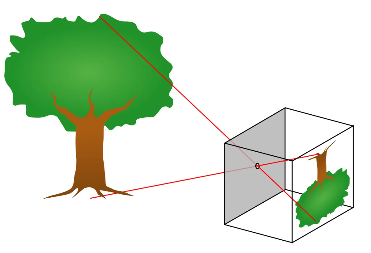
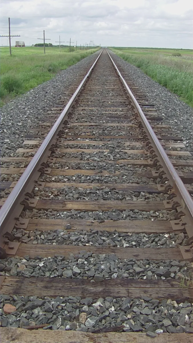
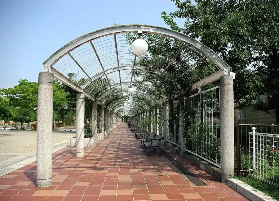
A camera squashes the 3D world onto a flat image. That squashing — perspective projection — is why railway lines meet in the distance and why a block twice as far looks half as wide. To guide a robot arm you must understand it in both directions: 3D → pixel (to predict where something will appear) and pixel → 3D (to tell the arm where to go). The second direction is only possible when you add one more fact, such as “the object is lying on the table”.
Concept
From 3D to pixels — and back to the table
1. The projection rule
For a point (X, Y, Z) in the camera frame (Z = distance straight ahead), the calibrated pinhole camera from Lesson 12 gives: u = fx·X/Z + cx and v = fy·Y/Z + cy. The division by Z is the whole story of perspective: double the distance and every offset from the image centre halves.
| Distance Z | A 50 mm block appears (fx = 900 px) |
|---|---|
| 250 mm | 180 px wide |
| 500 mm | 90 px wide |
| 1000 mm | 45 px wide |
| 2000 mm | 22.5 px wide |
2. One pixel is a whole ray
The points (100, 50, 500), (200, 100, 1000) and (400, 200, 2000) mm all land on the same pixel (820, 450). Going backwards, a pixel only tells you a *direction* — a ray from the camera — not a distance. To get a 3D point you need one more fact: the known size of the object, a depth sensor, a second camera, or a known surface like the table.
3. Back to the table: two good ways and one bad way
Ray meets plane
Turn the pixel into a ray with K⁻¹, rotate it into the table frame using the camera pose, and find where it hits the table (height 0). Needs K and the camera pose.
Homography
Put four tape marks on the table at known (X, Y) mm. Find them in the image once and let
cv.findHomographycompute a 3 × 3 matrix H. After that,cv.perspectiveTransformturns any table pixel into mm. Any two images of the same flat surface are related by a homography.One scale for the whole image (avoid!)
“1 px = 0.8 mm everywhere” is only true for a camera looking straight down at a flat table, with no distortion. With a tilted camera it is badly wrong away from where you measured it.
Visual
Visualise it: project points while changing Z
Switch to Perspective project mode: slide scene depth Z and focal length fx and watch the projected points move towards the principal point as Z grows. Educational pinhole model.
Interactive · Camera calibration lab · Educational

Intrinsics K map rays to pixels; bad fx / unmodeled distortion raise reprojection residual. Projection collapses Z — robots recover depth later. Estimates are educational, not a real OpenCV calibration runtime.
Code lab
Code lab: project, back-project and make a bird’s-eye view
The script uses the K from Lesson 12 (here fx = fy = 900, cx = 640, cy = 360) and a virtual camera 600 mm above the table, tilted 40° towards the arm. Eight blocks are placed at random on the table, projected to pixels with 0.5 px of detector noise, and then sent back to the table three ways.
"""Stage 11 L13 - Perspective and projection, with numbers you can check.

1) Project 3D points with the pinhole model (by hand and with cv.projectPoints)
2) Size shrinks as 1/Z, and one pixel is a whole ray (depth is lost)
3) Pixel -> table millimetres two ways: ray-plane intersection, and a homography
4) Bird's-eye view of a tilted table with cv.warpPerspective

Needs: opencv-python, numpy.   Run: python projection_lab.py
"""
import cv2 as cv
import numpy as np

K = np.array([[900.0, 0, 640], [0, 900.0, 360], [0, 0, 1]])   # from your Lesson 12 calibration
D = np.zeros(5)                                               # assume undistorted points here

# --- 1) project by hand vs OpenCV --------------------------------------------------------
P = np.array([[100.0, 50.0, 500.0]])                          # mm, in the camera frame
u = K[0, 0] * P[0, 0] / P[0, 2] + K[0, 2]
v = K[1, 1] * P[0, 1] / P[0, 2] + K[1, 2]
cvp, _ = cv.projectPoints(P, np.zeros(3), np.zeros(3), K, D)
print('1) Point (100, 50, 500) mm in the camera frame')
print(f'   by hand  u = 900*100/500 + 640 = {u:.1f}   v = 900*50/500 + 360 = {v:.1f}')
print(f'   OpenCV   u = {cvp[0,0,0]:.1f}   v = {cvp[0,0,1]:.1f}')

# --- 2) size vs distance, and the lost depth ------------------------------------------------
print('\n2) A 50 mm block seen at different distances')
for Z in (250, 500, 1000, 2000):
    w = K[0, 0] * 50 / Z
    print(f'   Z = {Z:4d} mm -> {w:6.1f} px wide')
print('   distance from size: Z = fx * 50 / width_px -> a 90 px wide block is', K[0, 0] * 50 / 90, 'mm away')
for s in (1, 2, 4):
    q = P * s
    pp, _ = cv.projectPoints(q, np.zeros(3), np.zeros(3), K, D)
    print(f'   point {q[0].astype(int)} -> pixel ({pp[0,0,0]:.1f}, {pp[0,0,1]:.1f})   <- same pixel, different depth')

# --- 3) a tilted camera above a table -----------------------------------------------------
# camera 600 mm above the table, tilted 40 deg towards the arm; table frame: X right, Y away, Z up
tilt = np.radians(40)
R_wc = np.array([[1, 0, 0],                          # columns = camera x, y, z axes in the table frame
                 [0, -np.cos(tilt), np.sin(tilt)],
                 [0, -np.sin(tilt), -np.cos(tilt)]])
C = np.array([0.0, -300.0, 600.0])                   # camera position on the table frame (mm)
R = R_wc.T                                           # table -> camera rotation
t = -R @ C
rvec, _ = cv.Rodrigues(R)

def to_pixels(pts_xy):
    pts = np.c_[pts_xy, np.zeros(len(pts_xy))].astype(np.float64)
    pp, _ = cv.projectPoints(pts, rvec, t, K, D)
    return pp.reshape(-1, 2)

rng = np.random.default_rng(13)
blocks = np.c_[rng.uniform(-250, 250, 8), rng.uniform(50, 450, 8)]
pix = to_pixels(blocks) + rng.normal(0, 0.5, (8, 2))          # detector noise 0.5 px

# 3a) ray-plane: back-project the pixel to a ray and intersect with Z = 0
def ray_to_table(uv):
    ray_cam = np.linalg.inv(K) @ np.array([uv[0], uv[1], 1.0])
    ray = R_wc @ ray_cam
    s = -C[2] / ray[2]
    return (C + s * ray)[:2]

# 3b) homography from four tape marks with known table positions
marks = np.array([[-300.0, 0], [300, 0], [300, 500], [-300, 500]])
H, _ = cv.findHomography(to_pixels(marks), marks)

# 3c) naive: one fixed mm-per-pixel scale measured at the table centre
centre_px = to_pixels(np.array([[0.0, 250.0]]))[0]
scale = 10.0 / np.linalg.norm(to_pixels(np.array([[10.0, 250.0]]))[0] - centre_px)

print('\n3) Camera 600 mm up, tilted 40 deg. Pixel -> table position error over 8 blocks')
err_ray, err_h, err_naive = [], [], []
for b, p in zip(blocks, pix):
    err_ray.append(np.linalg.norm(ray_to_table(p) - b))
    hb = cv.perspectiveTransform(p.reshape(1, 1, 2), H)[0, 0]
    err_h.append(np.linalg.norm(hb - b))
    naive = np.array([0.0, 250.0]) + (p - centre_px) * scale * np.array([1, -1])
    err_naive.append(np.linalg.norm(naive - b))
print(f'   ray + table plane (needs K and pose): mean {np.mean(err_ray):5.2f} mm, worst {np.max(err_ray):5.2f} mm')
print(f'   homography from 4 tape marks       : mean {np.mean(err_h):5.2f} mm, worst {np.max(err_h):5.2f} mm')
print(f'   one mm-per-pixel scale (naive)      : mean {np.mean(err_naive):5.1f} mm, worst {np.max(err_naive):5.1f} mm')

# 3d) height breaks the table-plane assumption
top = np.array([[100.0, 250.0, 60.0]])                      # top face of a 60 mm tall box
ptop, _ = cv.projectPoints(top, rvec, t, K, D)
guess = cv.perspectiveTransform(ptop.reshape(1, 1, 2), H)[0, 0]
print(f'   top of a 60 mm tall box at (100, 250): homography says ({guess[0]:.0f}, {guess[1]:.0f}) '
      f'-> {np.linalg.norm(guess - top[0, :2]):.0f} mm off (it assumes height 0)')

# --- 4) bird's-eye view ------------------------------------------------------------------
img = np.full((720, 1280, 3), 60, np.uint8)
grid = [np.array([[x, y] for x in range(-300, 301, 50)], float) for y in range(0, 501, 50)]
grid += [np.array([[x, y] for y in range(0, 501, 50)], float) for x in range(-300, 301, 50)]
for row in grid:
    cv.polylines(img, [to_pixels(row).astype(np.int32)], False, (200, 200, 200), 2)
mm_to_px = np.array([[1, 0, 300], [0, -1, 500], [0, 0, 1]], float)   # 1 px = 1 mm, origin bottom-left
top_view = cv.warpPerspective(img, mm_to_px @ H, (600, 500))
cv.imwrite('camera_view.png', img)
cv.imwrite('birds_eye.png', top_view)
print('\n4) saved camera_view.png (lines converge) and birds_eye.png (a square grid again)')
Output (tested with opencv-python 5.0)
1) Point (100, 50, 500) mm in the camera frame
   by hand  u = 900*100/500 + 640 = 820.0   v = 900*50/500 + 360 = 450.0
   OpenCV   u = 820.0   v = 450.0

2) A 50 mm block seen at different distances
   Z =  250 mm ->  180.0 px wide
   Z =  500 mm ->   90.0 px wide
   Z = 1000 mm ->   45.0 px wide
   Z = 2000 mm ->   22.5 px wide
   distance from size: Z = fx * 50 / width_px -> a 90 px wide block is 500.0 mm away
   point [100  50 500] -> pixel (820.0, 450.0)   <- same pixel, different depth
   point [ 200  100 1000] -> pixel (820.0, 450.0)   <- same pixel, different depth
   point [ 400  200 2000] -> pixel (820.0, 450.0)   <- same pixel, different depth

3) Camera 600 mm up, tilted 40 deg. Pixel -> table position error over 8 blocks
   ray + table plane (needs K and pose): mean  0.93 mm, worst  1.56 mm
   homography from 4 tape marks       : mean  0.93 mm, worst  1.56 mm
   one mm-per-pixel scale (naive)      : mean  37.3 mm, worst  73.4 mm
   top of a 60 mm tall box at (100, 250): homography says (111, 311) -> 62 mm off (it assumes height 0)

4) saved camera_view.png (lines converge) and birds_eye.png (a square grid again)
Reading the output
- By hand = OpenCV: u = 900·100/500 + 640 = 820 —
cv.projectPointsgives exactly the same. There is no magic inside. - Same pixel, three depths: scaling a point by 2 or 4 keeps its pixel. Depth is lost in a single image.
- Ray-plane and homography: both bring the blocks back within about 1 mm on average (worst 1.6 mm) — the leftover is the 0.5 px detector noise.
- One scale everywhere: 37 mm average and 73 mm worst error. On a tilted camera this is enough to miss a block completely.
- Tall box: the homography put the top of a 60 mm box 62 mm away from its real position, because it assumes height 0.
- Bird’s-eye view:
camera_view.pngshows the table grid as a trapezoid with converging lines;cv.warpPerspectivewith the same H turns it back into a square grid inbirds_eye.png(1 px = 1 mm).
import cv2 as cv, numpy as np
d = np.load('camera_calib.npz'); K, D = d['K'], d['D']     # from Lesson 12
marks_px = np.array([[312, 610], [968, 604], [842, 228], [430, 232]], np.float32)  # click/measure YOUR marks
marks_mm = np.array([[-300, 0], [300, 0], [300, 500], [-300, 500]], np.float32)   # where you stuck them
marks_px = cv.undistortPoints(marks_px.reshape(-1, 1, 2), K, D, P=K)   # remove lens distortion first
H, _ = cv.findHomography(marks_px, marks_mm)
np.save('table_H.npy', H)

block_px = cv.undistortPoints(np.array([[[700, 400]]], np.float32), K, D, P=K)   # detected block centre
print(cv.perspectiveTransform(block_px, H))                                      # -> [[[X_mm, Y_mm]]]
The pixel numbers above are only an example — replace them with the positions of your own tape marks. Undistort first: a homography is a straight-line mapping, and lens distortion bends straight lines.
Bench build: check “distance from size” with an ultrasonic sensor
Hold a 50 mm block (or a card of known width) in front of the camera, measure its width in pixels with your colour detector from Lesson 10, and compute Z = fx × 50 ÷ width. At the same time, an HC-SR04 ultrasonic sensor next to the camera measures the distance with sound. If the two agree within a few per cent, your fx and your detector are both good.
| HC-SR04 pin | Arduino UNO | Note |
|---|---|---|
| VCC | 5V | small 5 V sensor — fine on the UNO 5V pin |
| GND | GND | |
| TRIG | D9 | 10 µs pulse starts a measurement |
| ECHO | D10 | pulse length = time for the sound to go and return |
// Stage 11 L13 - Check "distance from size" with an ultrasonic sensor (HC-SR04)
// The camera estimates Z = fx * real_width / width_in_pixels. This sketch measures the
// same distance with sound, so you can compare the two in the Serial Monitor or from Python.
// Wiring: HC-SR04 VCC -> 5V, GND -> GND, TRIG -> D9, ECHO -> D10.
// The HC-SR04 is a small 5 V sensor (a few mA), fine on the UNO 5V pin. Nothing else is powered here.

const byte TRIG = 9, ECHO = 10;

long readMm() {
  digitalWrite(TRIG, LOW);
  delayMicroseconds(2);
  digitalWrite(TRIG, HIGH);                    // 10 us pulse starts one measurement
  delayMicroseconds(10);
  digitalWrite(TRIG, LOW);
  unsigned long us = pulseIn(ECHO, HIGH, 30000UL);   // give up after 30 ms (about 5 m)
  if (us == 0) return -1;                      // no echo
  return (long)(us * 0.343 / 2.0);             // speed of sound ~343 m/s at 20 C, out and back
}

void setup() {
  Serial.begin(115200);
  pinMode(TRIG, OUTPUT);
  pinMode(ECHO, INPUT);
}

void loop() {
  long sum = 0;
  byte good = 0;
  for (byte i = 0; i < 5; i++) {               // average 5 readings
    long d = readMm();
    if (d > 0) { sum += d; good++; }
    delay(60);                                 // let old echoes die out
  }
  if (good == 0) Serial.println(F("DIST none"));
  else { Serial.print(F("DIST ")); Serial.println(sum / good); }   // e.g. DIST 498
}Debugging
| Symptom | Likely cause | Fix |
|---|---|---|
| Positions good in the middle, bad at the edges | lens distortion not removed | Use cv.undistortPoints with K and D before the homography |
| Everything mirrored or rotated | tape marks listed in a different order in pixels and mm | List the four marks in the same order in both arrays |
| Tall objects land too far away | homography assumes height 0 | Use the bottom-centre of the object, not its top |
| Positions drift during the day | camera bumped or tripod sagging | Re-find the four marks (or detect them automatically) and recompute H |
| Size-based distance always 10% off | fx wrong, or real width wrong | Recalibrate (Lesson 12) and measure the object with calipers |
| Ultrasonic reads “none” or jumps | soft or angled target, or too close | Use a flat, hard card facing the sensor, at least a few cm away |
Real world
Projection in real systems
Robot picking from a table or conveyor: a fixed camera plus a table homography is a common way to turn detections into robot coordinates, as long as the parts lie flat. Wikipedia lists image rectification, image registration and augmented reality among the uses of homographies.
- Flattening a tilted photo: a photo of a page or a poster taken at an angle can be flattened with a homography from its four corners — the same
warpPerspectiveyou used (image rectification). - Augmented reality: once the homography of a flat surface is known, graphics can be drawn onto it with the correct perspective so they look part of the scene.
- Image registration: two photos of the same flat surface (for example, the table before and after the arm moved a block) can be aligned exactly and compared.
Think
Think about it
Think
Two points in front of the camera land on exactly the same pixel. What must be different about them — and what extra fact would let the robot choose the right one?
Experiment
Try it in the lab
About 45 minutes. You need your calibrated webcam (Lesson 12), masking tape, a ruler or measuring tape, and a few blocks. Bench part: Arduino UNO and an HC-SR04 sensor.
Experiment
Turn table pixels into millimetres
You will need
- `projection_lab.py` (opencv-python, numpy)
- Your `camera_calib.npz` from Lesson 12
- Masking tape, measuring tape, coloured blocks
- Camera calibration lab (browser), Perspective project mode
- Bench: Arduino UNO, HC-SR04, 4 jumper wires
Steps
- Run `projection_lab.py`. Change the tilt from 40° to 0° (looking straight down). What happens to the error of the single-scale method?
- Increase the detector noise from 0.5 to 2 px. How do the ray-plane and homography errors change?
- In the browser lab, use Perspective project mode: double Z and check that offsets from the principal point halve.
- Stick four tape marks on your real table, measure their positions in mm, and compute H for your camera.
- Place 5 blocks, measure their true positions with a tape, and compare with the homography result.
- Bench: compare the camera’s size-based distance with the HC-SR04 at 30, 50 and 80 cm.
Interactive · Camera calibration lab · Educational
Intrinsics K map rays to pixels; bad fx / unmodeled distortion raise reprojection residual. Projection collapses Z — robots recover depth later. Estimates are educational, not a real OpenCV calibration runtime.
- Straight-down cameras make one scale almost good enough; tilted cameras do not.
- Homography errors stay small across the table if distortion is removed first.
- Size-based distance and ultrasonic distance agree when fx and the object width are right.
Knowledge check
Check your understanding
Knowledge check
1. With fx = 900 px, a 50 mm block at Z = 1000 mm appears about…
2. Why can’t a single image give the 3D position of a point?
3. A homography from four tape marks maps pixels to table mm correctly for…
4. In the lab, using one mm-per-pixel scale with a tilted camera gave…
5. Before computing a homography on a real webcam you should…
Mini assignment
Hands-on assignment
Mini assignment
A pixel-to-millimetre map of the lab table
Build and test a homography that turns any table pixel from your camera into (X, Y) mm in the arm’s table frame.
Deliverables
- `table_H.npy` and the four tape-mark positions (pixels and mm).
- A bird’s-eye image of your table made with `cv.warpPerspective`.
- A table of 5 blocks: true mm, homography mm, and error.
- One paragraph: where on the table is the error largest, and why?
Do this, step by step
- Stick four tape marks on the table and measure their (X, Y) in mm from the arm’s base.
- Click or read their pixel positions and compute H; save it as
table_H.npy. - Make a bird’s-eye image of the table with
cv.warpPerspective. - Place 5 blocks, measure their true positions, and compare with the homography result.
- Write where the error is largest and why.
Stuck? Hints, one at a time
- The four marks must not be in a line; spread them near the table corners.
- Keep the points in the same order in both lists (pixels and mm), or H will be twisted.
- A homography is exact only for points on the table plane — a tall block’s top will be off.
Challenges (pick by level)
- 🟢 Beginner: Compute by hand where a point (50, −20, 400) mm lands with fx = fy = 900, cx = 640, cy = 360, and check with
cv.projectPoints. - 🟡 Intermediate: Add the size-based distance to your Lesson 10 colour detector and print it next to each box.
- 🟠 Advanced: Use six or more tape marks with
cv.findHomography(..., cv.RANSAC)and show it survives one wrongly-clicked mark. - 🔴 Expert: Compute the camera pose from the four marks with
cv.solvePnPand use the ray-plane method; compare with the homography. - ⚫ Research: Correct the tall-box error: if you know an object’s height h, intersect the ray with the plane Z = h instead of Z = 0, and test it on boxes of three heights.
Next step
A single image loses depth — so let’s measure it. In Lesson 14 — Depth and 3D Vision you get Z back with stereo cameras and depth sensors, and build a small 3D view of the table.
Sources
- Wikipedia — Pinhole camera model — projection y = f·x/x₃, principal point, the virtual image plane, homogeneous coordinates; the model ignores lens distortion, which grows towards the image edges.
- Wikipedia — Homography (computer vision)) — any two images of the same planar surface are related by a homography; uses in rectification, registration and augmented reality; OpenCV
findHomography/perspectiveTransform. - OpenCV 4.x — Camera Calibration — camera matrix K, distortion coefficients and
cv.projectPoints. - Photos: Wikimedia Commons (credits under each image).
Look back: Lesson 12: Camera Calibration. Next: Lesson 14: Depth & 3D Vision. Related: Stage 11 — Computer Vision, Stage 13 — Perception, Planning & Manipulation.
Self-attested for now — keep artifacts in your lab notebook.
Complete
Today's goal
0 of 1 done today
Mark this lesson complete when you have worked the experiment, knowledge check, and assignment (even roughly).