
Robot Perception, Planning & Manipulation · Lesson 07
Configuration Space for Manipulators
Est. 60–75 min
Why
Why this lesson matters
In Lesson 6 you learnt the big idea: plan the whole arm as one point moving through configuration space. Now we make that space real for manipulators. Real joints have limits. Some joints wrap around. The same gripper pose can be reached by several joint solutions. And an arm can hit itself. Each of these changes the shape of C-space, and a planner that ignores them will produce motions that are long, impossible or dangerous.
In the code lab you will measure each effect on a desk arm: the wrap-around distance, how much reach joint limits remove, how to choose between IK solutions by C-space distance, how much of a 3-link arm’s C-space is self-collision — and how random sampling estimates it without a full grid. On the bench, an Arduino computes both IK solutions for a typed target, rejects the ones outside the joint limits, and moves to the nearest one.
Concept
Joint space, wrap-around, limits, IK branches and self-collision
1. Joint space is the arm’s configuration space
For a robot arm, the joint values are the natural coordinates of a configuration. The set of all joint values is called the joint space. Forward kinematics maps a point in joint space to a gripper pose; inverse kinematics goes back the other way. A motion planner for an arm almost always works in joint space, because every point there is one complete, unambiguous pose of the robot.
2. Wrap-around: lines, circles and the torus
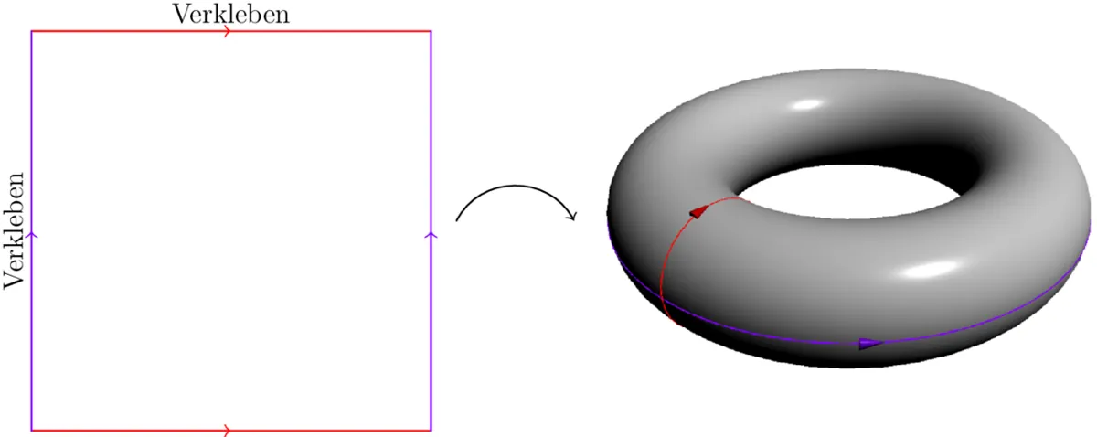
A revolute joint that can turn without limit (a continuous joint) has a C-space that is a circle: 179° and −179° are only 2° apart. Two such joints give a circle × circle — a torus, the surface of a doughnut. Imagine the (q1, q2) square from Lesson 6: glue its left edge to its right edge, and its top edge to its bottom edge, and you get a torus. A planner on a continuous joint must measure distance the short way round.
| Joint type | C-space of that joint | Distance from 170° to −170° |
|---|---|---|
| Continuous revolute (no stops) | a circle | 20° (the short way round) |
| Revolute with stops (most arm joints, hobby servos) | a line segment, e.g. 0°…180° | the long way, or not possible at all if outside the range |
| Prismatic (linear slide) | a line segment, e.g. 0…300 mm | — |
3. Joint limits cut the box
Most real joints have mechanical stops, cable limits or software limits. Those turn the C-space into a box (q_min ≤ q ≤ q_max for each joint). Anything outside the box simply does not exist for the planner. Good practice is to keep a small soft limit margin (say 5°) inside the mechanical stop, so the servo never drives hard into its end. In our script, typical hobby-servo limits leave the tip only about half of the area it could reach with no limits.
4. Several IK solutions = several points in C-space
For a 2-link arm, most reachable tip positions have two IK solutions: elbow + and elbow −. They are two different points in C-space that put the tip at the same place. A 6-DOF arm usually has more. The planner must choose one, and the choice matters: a solution outside the joint limits is useless; a solution in collision is useless; among the rest, the one nearest in C-space to the current pose usually gives the shortest and safest motion. Near full stretch the solutions come together — the singularity you met in Stage 8.
5. Self-collision
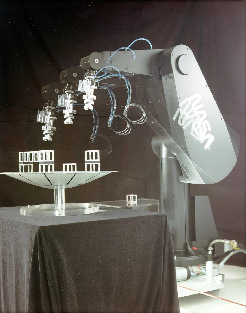
An arm with three or more links can fold back and hit itself — the wrist link against the upper arm, the gripper against the base. These configurations are also C-obstacles, even with an empty table. Planners check every pair of links that are not neighbours (neighbouring links always touch at their shared joint, so those pairs are skipped). In our script, about 15% of the 3-link arm’s (q2, q3) space is self-collision.
6. When grids give up, sample
A grid with 3° steps on 6 joints has trillions of cells. But if you pick configurations at random and check each one, the fraction you find in collision gets close to the true fraction quickly — and the error depends on how many samples you take, not on how many joints the arm has. That simple fact is the seed of the sampling-based planners in Lessons 9 and 10.
Visual
Visualise it: the shape of an arm’s C-space
Every pose of the arm is one point in joint space. Joint limits make the space a box, continuous joints make it wrap around, and obstacles and self-collision carve forbidden regions out of it. (Educational explorer, not an industrial motion planner.)
Interactive · Configuration space explorer · Educational 2R


Educational C-space sketch for planar 2R — not OMPL / not MoveIt / not 6DOF C-space.
Code lab
Code lab: measure the shape of an arm’s C-space
manipulator_cspace_lab.py uses the same desk arm (links 15 cm and 12 cm, plus an 8 cm wrist link in parts 4–5). Five parts: (1) wrap-around distance; (2) how joint limits shrink the reachable tip area; (3) choosing between IK solutions by C-space distance; (4) self-collision on a 5° grid; (5) estimating the same fraction by random sampling. Plain Python 3. Run python3 manipulator_cspace_lab.py.
"""manipulator_cspace_lab.py — Stage 13 L07 (AIHUB STATION lab)

Configuration space for real manipulators: wrap-around joints, joint limits,
several IK solutions, self-collision, and why we start to SAMPLE.
Top view, example values in metres: links 0.15 m and 0.12 m (+ a 0.08 m wrist in part 4).
Run:  python3 manipulator_cspace_lab.py
"""
import math, random

L1, L2, L3 = 0.15, 0.12, 0.08

def wrap(a):                     # angle to (-180, 180]
    a = (a + 180.0) % 360.0 - 180.0
    return 180.0 if a == -180.0 else a

def joint_dist(a, b, continuous):
    d = abs(a - b)
    return min(d, 360 - d) if continuous else d

def fk(qs, lens):
    x = y = th = 0.0; pts = [(0.0, 0.0)]
    for q, L in zip(qs, lens):
        th += math.radians(q); x += L*math.cos(th); y += L*math.sin(th); pts.append((x, y))
    return pts

def ik2(x, y):
    c2 = (x*x + y*y - L1*L1 - L2*L2) / (2*L1*L2)
    if abs(c2) > 1: return []
    out = []
    for s in (+1, -1):
        q2 = s*math.acos(c2)
        q1 = math.atan2(y, x) - math.atan2(L2*math.sin(q2), L1 + L2*math.cos(q2))
        out.append((wrap(math.degrees(q1)), math.degrees(q2)))
    return out

# ---------- 1. wrap-around ----------
print("1. A continuous base joint wraps around (C-space is a circle, not a line)")
a, b = 170.0, -170.0
print(f"   from {a:.0f} deg to {b:.0f} deg: as a line {joint_dist(a, b, False):.0f} deg, as a circle {joint_dist(a, b, True):.0f} deg")
print("   Two continuous joints: circle x circle = a torus (a doughnut surface).")
print("   A hobby servo (0..180 deg) does NOT wrap: it must go the long way, or cannot go at all.")

# ---------- 2. joint limits ----------
print("\n2. Joint limits shrink what the tip can reach (2-link arm, tip sampled on a 1 cm grid)")
def reachable_cells(q1_lim, q2_lim, step=1.0):
    cells = set()
    q1 = q1_lim[0]
    while q1 <= q1_lim[1]:
        q2 = q2_lim[0]
        while q2 <= q2_lim[1]:
            x, y = fk((q1, q2), (L1, L2))[-1]
            cells.add((round(x*100), round(y*100)))
            q2 += step
        q1 += step
    return len(cells)
full = reachable_cells((-180, 179), (-180, 179))
for name, l1, l2 in (("no limits", (-180, 179), (-180, 179)),
                     ("q1 -90..90, q2 -150..150", (-90, 90), (-150, 150)),
                     ("hobby servos: q1 -90..90, q2 0..150", (-90, 90), (0, 150))):
    n = reachable_cells(l1, l2)
    print(f"   {name:36s}: {n:4d} tip cells ({100*n/full:.0f}% of the no-limit area)")

# ---------- 3. several IK solutions = several C-space points ----------
print("\n3. One tip position, two arm poses (elbow + and elbow -)")
current = (10.0, 60.0)
for tip in ((0.20, 0.05), (0.05, 0.22), (0.268, 0.0)):
    sols = ik2(*tip)
    if not sols:
        print(f"   tip {tip}: unreachable"); continue
    desc = []
    for q in sols:
        d = math.hypot(joint_dist(q[0], current[0], True), joint_dist(q[1], current[1], False))
        desc.append((d, q))
    desc.sort()
    txt = "; ".join(f"q=({q[0]:.1f}, {q[1]:.1f}) distance {d:.1f} deg" for d, q in desc)
    print(f"   tip ({tip[0]:.3f}, {tip[1]:.3f}) m: {txt}")
print(f"   (current pose q={current}). Pick the nearer one in C-space -> smaller, safer motion.")
print("   Near full stretch (0.268 of 0.27 m) the two poses almost merge; at full stretch they are one pose: a singularity (Stage 8).")

# ---------- 4. self-collision for a 3-link arm ----------
print("\n4. Self-collision: can the wrist link hit the upper arm? (3 links, capsule radius 1.5 cm)")
def seg_seg_dist(p1, p2, p3, p4):
    def pt_seg(p, a, b):
        ax, ay = a; bx, by = b
        L = (bx-ax)**2 + (by-ay)**2
        s = 0 if L == 0 else max(0, min(1, ((p[0]-ax)*(bx-ax) + (p[1]-ay)*(by-ay)) / L))
        return math.hypot(ax + s*(bx-ax) - p[0], ay + s*(by-ay) - p[1])
    return min(pt_seg(p1, p3, p4), pt_seg(p2, p3, p4), pt_seg(p3, p1, p2), pt_seg(p4, p1, p2))
def self_hit(q2, q3, r=0.015):
    pts = fk((0.0, q2, q3), (L1, L2, L3))
    return seg_seg_dist(pts[0], pts[1], pts[2], pts[3]) < 2*r
STEP = 5
total = hits = 0
for q2 in range(-180, 180, STEP):
    for q3 in range(-180, 180, STEP):
        total += 1; hits += self_hit(q2, q3)
print(f"   q2, q3 on a {STEP} deg grid: {hits} of {total} poses ({100*hits/total:.1f}%) are self-collisions")
print(f"   e.g. q=(0, 150, 150): {'HIT' if self_hit(150, 150) else 'free'};  q=(0, 90, 90): {'HIT' if self_hit(90, 90) else 'free'};  q=(0, 30, 30): {'HIT' if self_hit(30, 30) else 'free'}")
print("   (Neighbouring links always touch at their shared joint, so planners skip those pairs.)")

# ---------- 5. sampling instead of a full grid ----------
print("\n5. Estimating the self-collision fraction by random SAMPLING")
random.seed(7)
for n in (100, 1000, 10000):
    h = sum(self_hit(random.uniform(-180, 180), random.uniform(-180, 180)) for _ in range(n))
    print(f"   {n:6d} random samples: {100*h/n:5.1f}% self-collision")
print("   1000 samples already land within 1% of the full 5 deg grid (15.0%). The sampling error depends on\n   the number of samples, NOT on the number of joints; a grid needs (360/step)^joints cells.")
print("   This is the idea behind sampling-based planners (L9, L10).")
Output (run with python3 manipulator_cspace_lab.py)
1. A continuous base joint wraps around (C-space is a circle, not a line)
   from 170 deg to -170 deg: as a line 340 deg, as a circle 20 deg
   Two continuous joints: circle x circle = a torus (a doughnut surface).
   A hobby servo (0..180 deg) does NOT wrap: it must go the long way, or cannot go at all.

2. Joint limits shrink what the tip can reach (2-link arm, tip sampled on a 1 cm grid)
   no limits                           : 2380 tip cells (100% of the no-limit area)
   q1 -90..90, q2 -150..150            : 1586 tip cells (67% of the no-limit area)
   hobby servos: q1 -90..90, q2 0..150 : 1164 tip cells (49% of the no-limit area)

3. One tip position, two arm poses (elbow + and elbow -)
   tip (0.200, 0.050) m: q=(-21.1, 81.1) distance 37.5 deg; q=(49.1, -81.1) distance 146.4 deg
   tip (0.050, 0.220) m: q=(47.9, 67.1) distance 38.5 deg; q=(106.5, -67.1) distance 159.6 deg
   tip (0.268, 0.000) m: q=(-6.2, 14.0) distance 48.7 deg; q=(6.2, -14.0) distance 74.1 deg
   (current pose q=(10.0, 60.0)). Pick the nearer one in C-space -> smaller, safer motion.
   Near full stretch (0.268 of 0.27 m) the two poses almost merge; at full stretch they are one pose: a singularity (Stage 8).

4. Self-collision: can the wrist link hit the upper arm? (3 links, capsule radius 1.5 cm)
   q2, q3 on a 5 deg grid: 778 of 5184 poses (15.0%) are self-collisions
   e.g. q=(0, 150, 150): HIT;  q=(0, 90, 90): free;  q=(0, 30, 30): free
   (Neighbouring links always touch at their shared joint, so planners skip those pairs.)

5. Estimating the self-collision fraction by random SAMPLING
      100 random samples:  22.0% self-collision
     1000 random samples:  15.7% self-collision
    10000 random samples:  15.8% self-collision
   1000 samples already land within 1% of the full 5 deg grid (15.0%). The sampling error depends on
   the number of samples, NOT on the number of joints; a grid needs (360/step)^joints cells.
This is the idea behind sampling-based planners (L9, L10).Try it: move the q1 and q2 sliders and watch the arm and its single point in C-space. The blocked region here is a simplified box-shaped C-obstacle. Find two different poses that put the tip near the same spot. (Educational explorer, not an industrial motion planner.)
Interactive · Configuration space explorer · Educational 2R
Educational C-space sketch for planar 2R — not OMPL / not MoveIt / not 6DOF C-space.
Bench build: choose the right IK solution inside the joint limits
ik_choice_limits.ino reads a tip target “x y” in millimetres from the Serial Monitor. It computes both IK solutions, prints them, rejects any outside the soft joint limits (q1 −85…85°, q2 5…145°), and moves — slowly and with both joints synchronised — to the valid solution nearest to the current pose. If nothing is valid, it does not move. That is a tiny version of what a real planner does before it even starts searching.
| Part | Connection | Note |
|---|---|---|
| Shoulder servo (SG90-class) | signal → D9 | servo1 = q1 + 90° |
| Elbow servo (SG90-class) | signal → D10 | servo2 = q2 (elbow bends one way only) |
| Servo supply | red → +5–6 V, brown → supply GND | separate supply (about 2 A); supply GND joined to UNO GND |
| USB | UNO to laptop | Serial Monitor at 115200, “Newline” line ending |
// ik_choice_limits.ino — Stage 13 L07 (AIHUB STATION lab)
// Type a tip target "x y" in millimetres into the Serial Monitor (115200, newline).
// The UNO computes BOTH inverse-kinematics solutions (elbow + and elbow -),
// throws away any that break the joint limits, picks the one NEAREST to the
// current pose in configuration space, and moves there slowly.
//
// Wiring (Arduino UNO):
//   Shoulder servo signal -> D9, elbow servo signal -> D10
//   Servo red/brown -> SEPARATE 5-6 V supply (about 2 A), NOT the UNO 5V pin
//   Supply GND joined to UNO GND (common ground)
//
// Joint angles q (degrees) to servo angles (calibrate on YOUR arm first):
//   servo1 = q1 + 90   so q1 limits -90..90  map to servo 0..180
//   servo2 = q2        so q2 limits   0..150 map to servo 0..150
// We keep a 5 degree safety margin inside each limit (soft limits).
#include <Servo.h>
#include <math.h>

const float L1 = 150.0, L2 = 120.0;           // link lengths in mm
const float Q1_MIN = -90 + 5, Q1_MAX = 90 - 5; // soft limits (deg)
const float Q2_MIN = 0 + 5,   Q2_MAX = 150 - 5;
const float STEP_DEG = 1.0;                    // per 15 ms -> about 66 deg/s

Servo s1, s2;
float q1 = 0, q2 = 90;                         // start pose (deg)

bool inLimits(float a, float b) {
  return a >= Q1_MIN && a <= Q1_MAX && b >= Q2_MIN && b <= Q2_MAX;
}

void writeJoints() {
  s1.write(constrain((int)(q1 + 90.5), 0, 180));
  s2.write(constrain((int)(q2 + 0.5), 0, 180));
}

void moveTo(float t1, float t2) {               // synchronised slow move
  float d1 = t1 - q1, d2 = t2 - q2;
  int steps = max(1, (int)ceil(max(fabs(d1), fabs(d2)) / STEP_DEG));
  float a = q1, b = q2;
  for (int i = 1; i <= steps; i++) {
    q1 = a + d1 * i / steps; q2 = b + d2 * i / steps;
    writeJoints(); delay(15);
  }
}

void setup() {
  Serial.begin(115200);
  s1.attach(9); s2.attach(10);
  writeJoints();
  Serial.println(F("Type a tip target in mm, e.g.  200 50"));
}

void loop() {
  if (!Serial.available()) return;
  float x = Serial.parseFloat(), y = Serial.parseFloat();
  while (Serial.available()) Serial.read();      // drop the rest of the line

  float c2 = (x*x + y*y - L1*L1 - L2*L2) / (2*L1*L2);
  Serial.print(F("target (")); Serial.print(x); Serial.print(F(", ")); Serial.print(y); Serial.println(F(") mm"));
  if (c2 > 1 || c2 < -1) { Serial.println(F("  out of reach: not moving")); return; }

  float best1 = 0, best2 = 0, bestDist = 1e9;
  for (int s = 1; s >= -1; s -= 2) {
    float b = s * acos(c2);
    float a = atan2(y, x) - atan2(L2 * sin(b), L1 + L2 * cos(b));
    float qa = a * 180.0 / PI, qb = b * 180.0 / PI;
    Serial.print(s > 0 ? F("  elbow +: q=(") : F("  elbow -: q=("));
    Serial.print(qa, 1); Serial.print(F(", ")); Serial.print(qb, 1); Serial.print(F(")"));
    if (!inLimits(qa, qb)) { Serial.println(F("  outside joint limits")); continue; }
    float d = sqrt((qa - q1)*(qa - q1) + (qb - q2)*(qb - q2));  // C-space distance
    Serial.print(F("  ok, distance ")); Serial.println(d, 1);
    if (d < bestDist) { bestDist = d; best1 = qa; best2 = qb; }
  }
  if (bestDist > 1e8) { Serial.println(F("  no solution inside the limits: not moving")); return; }
  Serial.print(F("  moving to q=(")); Serial.print(best1, 1); Serial.print(F(", ")); Serial.print(best2, 1); Serial.println(F(")"));
  moveTo(best1, best2);
}Type a tip target in mm, e.g. 200 50
target (200.00, 50.00) mm
elbow +: q=(-21.1, 81.1) ok, distance 22.9
elbow -: q=(49.1, -81.1) outside joint limits
moving to q=(-21.1, 81.1)
target (-100.00, 150.00) mm
elbow +: q=(82.3, 97.0) ok, distance 104.6
elbow -: q=(165.0, -97.0) outside joint limits
moving to q=(82.3, 97.0)
target (300.00, 0.00) mm
out of reach: not movingDebugging
| Symptom | Likely cause | Fix |
|---|---|---|
| Continuous joint spins the long way round | angle difference not wrapped | Use the short-way distance: min(|a−b|, 360 − |a−b|) |
| IK answer the servo cannot reach | joint limits not checked | Check every solution against limits before using it |
| Arm makes a big swing for a small tip move | IK chose the far branch | Pick the solution nearest in C-space to the current pose |
| Wrist hits the upper arm on an empty table | self-collision not checked | Check all non-neighbouring link pairs |
| Servo buzzes at one end | command at or past the mechanical stop | Add a soft-limit margin; re-calibrate the offset |
| Sampling estimate jumps around | too few samples | Use more samples; fix the random seed while debugging |
Real world
Configuration space in real arms
- Robot models: before a planner can search, someone must tell it each joint’s type and range. A wrong range in the model means the planner searches the wrong C-space — often the cause of “impossible” plans.
- Arms with several IK branches: elbow up or down, wrist flipped or not — choosing the branch before planning decides whether the motion is short and safe or long and awkward.
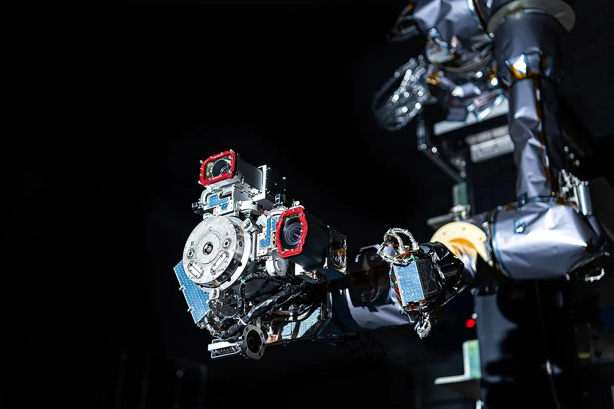
- Space arms: with long links, many joints and costly mistakes, self-collision and joint-limit checks are part of every motion.
- Your lab: write down each joint’s type and limits before writing any planner code. It takes five minutes and prevents most bench crashes.
Think
Think about it
Think
A 6-DOF arm has a continuous last joint (the gripper can spin freely), but its cable can only twist 2 full turns before it is damaged. Is that joint a circle or a line in C-space?
Experiment
Try it in the lab
About 60 minutes. Python 3 for the script; Arduino UNO and a 2-servo arm with its own 5–6 V supply for the bench.
Experiment
Map the limits, branches and self-collisions of your arm
You will need
- `manipulator_cspace_lab.py` (Python 3, no libraries)
- Configuration-space explorer (in your browser)
- Arduino UNO, 2 × SG90-class servos on a 2-link arm, separate 5–6 V supply, jumper wires, ruler
Steps
- Run the script. In part 2, try q2 limits of −150…0 instead of 0…150. Is the area the same? Why?
- In part 3, change the current pose to (60, −60). Which IK branch is chosen now?
- In part 4, make the capsule radius 2.5 cm. How does the self-collision fraction change?
- In part 5, run with 5 different seeds at 100 samples. How much do the answers spread?
- Bench: measure your servos’ real end stops and set the soft limits 5° inside them.
- Bench: type five targets, including one out of reach and one that needs the far side. Record which solutions are rejected and why.
Interactive · Configuration space explorer · Educational 2R
Educational C-space sketch for planar 2R — not OMPL / not MoveIt / not 6DOF C-space.
The shape of C-space comes from the robot itself: joint types, limits, IK branches and its own links. Get these right first; every planner in the next lessons depends on them.
Knowledge check
Check your understanding
Knowledge check
1. For an arm, the set of all joint values is called…
2. A continuous revolute joint has a C-space shaped like…
3. Two continuous joints together give a C-space shaped like…
4. On a continuous joint, the distance from 170° to −170° is…
5. Two IK solutions reach the same tip. A good planner usually picks…
6. Why keep a soft limit a few degrees inside the mechanical stop?
7. Self-collision means…
8. Why does random sampling help for a 6-DOF arm?
Mini assignment
Hands-on assignment
Mini assignment
A C-space data sheet for your arm
Describe your desk arm’s configuration space completely: joint types, limits, IK branches and self-collisions.
Deliverables
- A table of every joint: type (continuous / revolute with limits / prismatic), mechanical limits measured on the bench, and your soft limits.
- The reachable tip area with your limits, from a modified part 2 of the script, and a sketch of that area on graph paper.
- A bench log from `ik_choice_limits.ino` for at least five targets, with your explanation for each rejected solution.
- If your arm has 3 or more joints: the self-collision fraction from sampling, and two example self-colliding poses.
Do this, step by step
- Run
manipulator_cspace_lab.pyand look at the joint-limit and wrap-around results. - Write the soft limits for your arm a few degrees inside each mechanical stop.
- Test the 170° → −170° move with
joint_dist()for a continuous joint and for a limited joint. - Pick one target and compare both IK solutions (elbow up / elbow down) against your limits.
- Bench: upload
ik_choice_limits.ino, send targets in mm and log which IK solution it chooses and which it refuses.
Stuck? Hints, one at a time
- For a continuous joint, the shortest move from 170° to −170° is 20°, not 340°. Use
wrap(). - If both IK solutions are refused, check
Q1_MIN/Q1_MAXandQ2_MIN/Q2_MAXbefore blaming the IK. self_hit()uses a link radius of 1.5 cm. If your links are thicker, raise it.
Challenges (pick by level)
- 🟢 Beginner: Cut out a paper square, mark (q1, q2) on it, and roll it into a tube and then a torus (or just bend it). Mark where 179° and −179° meet.
- 🟡 Intermediate: Make the A* planner from Lesson 6 wrap around on q1 (a continuous base). Compare paths from 170° to −170° with and without wrap-around.
- 🟠 Advanced: Add a wrist joint to
ik_choice_limits.inowith a fixed gripper angle, so each target has up to two solutions with a wrist angle. Check all three joint limits. - 🔴 Expert: Estimate the self-collision fraction of a 6-joint planar chain by sampling. How many samples do you need for ±1%?
- ⚫ Research: Read how robot description files encode joint types and limits and how a motion planner reads them. Write one page on what goes wrong if a joint is described as continuous but is really cable-limited.
Next step
You now know what C-space looks like for a real arm. In Lesson 8 — Collision-Free Motion you will check whole motions, not just poses: how finely to check between waypoints, how to pad, and how to make sure nothing is missed between two safe poses.
Look back: Lesson 6: Path Planning vs Motion Planning. Next: Lesson 8: Collision-Free Motion. Related: Stage 8 — Kinematics & IK.
Sources
- Wikipedia — Configuration space (physics)) — robotic arm section: joint parameters as generalized coordinates, “joint space”, FK/IK as maps; note that some robotics texts use the term for reachable end-effector poses.
- Wikipedia — Motion planning — C-space of an N-joint arm is N-dimensional; C-free tested with forward kinematics and collision detection; grids grow exponentially; sampling-based planners for high dimensions.
- Arduino Servo library (GitHub) — controlling RC hobby servos.
- Photos: Wikimedia Commons (credits under each image).
Self-attested for now — keep artifacts in your lab notebook.
Complete
Today's goal
0 of 1 done today
Mark this lesson complete when you have worked the experiment, knowledge check, and assignment (even roughly).