
Robot Simulation & Digital Twin · Lesson 10
Simulated Sensors
Est. 55–70 min
Why
Why this lesson matters
The physics engine always knows the true state: exact angles, exact distances. A real sensor never does. It rounds to its resolution, adds noise, has a slowly wandering bias, can only see between a minimum and maximum range, updates only so many times a second, and arrives late. A simulated sensor takes the truth and adds these effects on purpose, so your code is tested against the same messy data it will meet on the bench.
In this chapter you will build each effect in Python, watch a small gyro bias turn into 17° of drift, see a delay make a calm controller go wild, and then measure the real noise of your own sensor with an Arduino and paste it into a simulator-style <noise> block.
Concept
How a simulator fakes a sensor — honestly
1. The recipe: reading = truth + effects
Think of a weighing scale at a sabzi mandi. The true weight of the tomatoes is one number. The scale shows it rounded to 5 g (resolution), the needle shakes a little (noise), it reads 10 g even when empty if nobody zeroed it (bias), it cannot weigh a truck (range), and the needle takes a second to settle (delay). Every robot sensor has the same five problems.
| Effect | What it looks like | How the simulator adds it |
|---|---|---|
| Resolution (quantisation) | readings jump in steps | round truth to the sensor’s step size |
| Noise | reading shakes around the truth | add a random Gaussian number each sample (stddev) |
| Bias | reading is off by a constant amount | add a fixed offset (drawn once, bias_mean / bias_stddev) |
| Range limits and dropouts | too near or too far → no reading | return inf or nothing outside min/max, or randomly |
| Update rate and latency | new data only every so often, and late | publish at <update_rate>, delay the message |
2. How SDF describes noise
Gazebo’s SDF format has a <noise> element with types none, gaussian and gaussian_quantized. Its settings include mean, stddev, bias_mean, bias_stddev, slowly wandering “dynamic bias” settings, and precision (the step size for the quantised type). Gazebo sensors also have <update_rate>; the Gazebo lidar tutorial uses 10 Hz with a range of 0.08 to 10 m.
<angular_velocity>
  <z>
    <noise type="gaussian">
      <mean>0.0</mean>
      <stddev>0.01</stddev>      <!-- rad/s shake on every sample -->
      <bias_mean>0.005</bias_mean>  <!-- rad/s constant offset -->
      <bias_stddev>0.001</bias_stddev>
    </noise>
  </z>
</angular_velocity>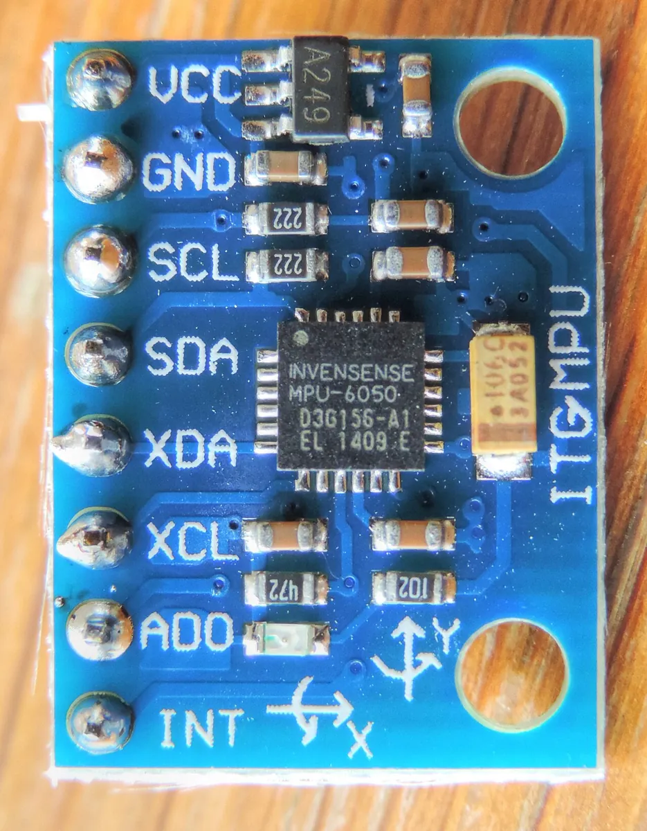
3. Sensors your arm and lab will use
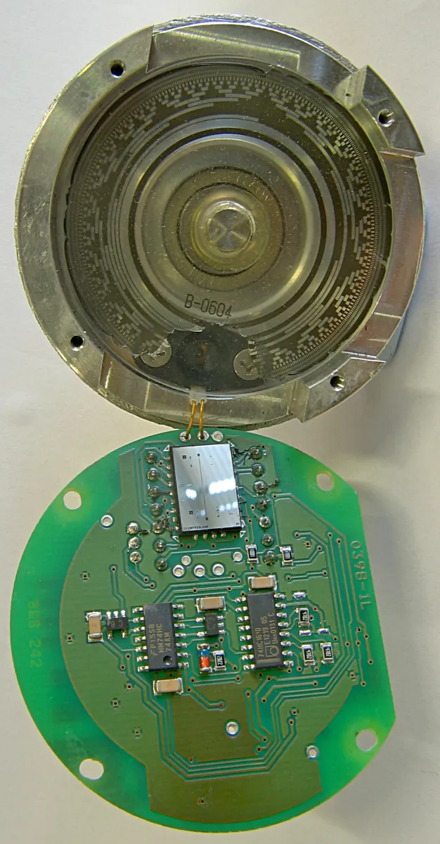
- Joint encoder or pot: angle → rounded to its resolution, small noise. In ROS 2 these become
sensor_msgs/JointState. - IMU: orientation, angular velocity (rad/s) and linear acceleration (m/s², not g). The ROS
sensor_msgs/Imumessage also carries covariance fields — an all-zero covariance means “unknown”. - Range (ultrasonic, ToF, lidar): distance with min/max range; returns nothing or infinity outside it.
- Contact: true/false when two collision shapes touch (Lesson 8).
- Camera: an image rendered from the scene, with lighting and lens effects (Stage 11).
Visual
Visualise it: truth, noise and delay
Sensor simulation lab: the true value, plus noise you control, for an encoder, toy IMU, range ray and camera pixel. (Educational toy, not real sensor drivers.)
Interactive · Sensor simulation lab · Educational

Reports joint angle from sim truth + optional noise. Educational — not a real AS5048 / magnetic encoder driver.
Sensor
Joint encoder
Reading
43.5°
Model
truth+noise
Educational sensor stubs — not ROS sensor_msgs, not Gazebo plugins, not live cameras/IMUs. Use noise & latency sliders to feel the sim-to-real gap.
Code lab
Code lab: build five sensor effects
sensor_sim_lab.py builds the five effects one by one using only the Python standard library. The random seed is fixed, so you get the same output every time. All sensor values are examples — later you will replace them with your measured numbers. Run python3 sensor_sim_lab.py.
"""Simulated sensors lab (Stage 12, Lesson 10) - Python 3 standard library only.

A simulator knows the TRUE state. A simulated sensor must report what a REAL
sensor would: rounded to its resolution, noisy, biased, limited in range,
updated only so often, and a little late. This script builds each effect.

  1. Encoder / pot quantisation: how fine can the reading be?
  2. Gaussian noise + bias (the SDF <noise> model) on a gyro -> heading drift
  3. A range sensor with min/max range, noise and dropouts
  4. Latency: the same P controller with 0, 40, 80 and 120 ms sensor delay
  5. Update rate: how far does the robot move between two readings?
All sensor numbers are EXAMPLES - measure or read your own sensor's datasheet.
"""
import math
import random

rng = random.Random(10)          # fixed seed -> same output every run

print("=== 1. Quantisation: the reading can only take certain values ===")
truth = 45.123
for name, steps, span in [("12-bit magnetic encoder", 4096, 360.0),
                          ("10-bit ADC on a 270 deg pot", 1024, 270.0),
                          ("hobby encoder, 20 slots", 20, 360.0)]:
    lsb = span / steps
    reading = round(truth / lsb) * lsb
    print(f"{name:>28}: step {lsb:6.3f} deg -> truth {truth} reads {reading:7.3f} (error {reading - truth:+.3f})")
print("-> a perfect float angle from the simulator is MORE precise than any real sensor.")

print()
print("=== 2. Gyro with SDF-style noise: stddev 0.01 rad/s, bias 0.005 rad/s ===")
STD, BIAS, RATE = 0.01, 0.005, 100.0   # example values, rad/s and Hz
dt = 1.0 / RATE
for label, std, bias in [("perfect gyro", 0.0, 0.0), ("noise only", STD, 0.0), ("noise + bias", STD, BIAS)]:
    heading = 0.0                                    # robot is standing still: true rate 0
    marks = []
    for k in range(1, int(60 * RATE) + 1):
        measured = 0.0 + bias + rng.gauss(0.0, std)
        heading += measured * dt                     # integrate rate -> angle
        if k % int(20 * RATE) == 0:
            marks.append(math.degrees(heading))
    print(f"{label:>14}: heading after 20/40/60 s = " + " / ".join(f"{m:+6.2f} deg" for m in marks))
print("-> random noise averages out a bit; a small constant BIAS grows forever")
print("   (0.005 rad/s x 60 s = 0.3 rad = 17 deg). Real IMUs drift exactly like this.")

print()
print("=== 3. Range sensor: min 0.02 m, max 4.0 m, noise 3 mm, 2 % dropouts ===")
def range_sensor(true_d):
    if rng.random() < 0.02:
        return None                                  # no echo this time
    if true_d < 0.02 or true_d > 4.0:
        return math.inf                              # out of range
    return round(true_d + rng.gauss(0.0, 0.003), 3)
for d in [0.01, 0.10, 0.50, 2.00, 5.00]:
    reads = [range_sensor(d) for _ in range(200)]
    good = [r for r in reads if r is not None and r != math.inf]
    inf = sum(1 for r in reads if r == math.inf)
    drop = sum(1 for r in reads if r is None)
    if good:
        mean = sum(good) / len(good)
        sd = (sum((g - mean) ** 2 for g in good) / len(good)) ** 0.5
        print(f"true {d:4.2f} m: mean {mean:.4f} m, spread {sd * 1000:.1f} mm, dropouts {drop}/200")
    else:
        print(f"true {d:4.2f} m: out of range ({inf} x inf), dropouts {drop}/200")
print("-> your code must handle inf and missing readings, or the real robot crashes.")

print()
print("=== 4. Latency: joint P controller, Kp 15 /s, step 0 -> 1.0 rad ===")
KP, DT = 15.0, 0.001
for delay_ms in [0, 40, 80, 120]:
    n_delay = int(delay_ms / 1000 / DT)
    history = [0.0] * (n_delay + 1)                 # old measurements waiting to arrive
    q, peak, t_settle = 0.0, 0.0, None
    for k in range(int(3.0 / DT)):
        history.append(q)
        q_seen = history.pop(0)                     # what the controller sees (late)
        q += KP * (1.0 - q_seen) * DT               # joint moves at the commanded speed
        peak = max(peak, q)
        if abs(q - 1.0) > 0.02:
            t_settle = None
        elif t_settle is None:
            t_settle = k * DT
    s = f"settles {t_settle:.2f} s" if t_settle is not None else "does NOT settle in 3 s"
    print(f"delay {delay_ms:3d} ms: overshoot {max(0.0, peak - 1.0) * 100:5.1f} %, {s}, q(3 s) = {q:.3f}")
print(f"-> Kp x delay must stay well below pi/2 (here limit {math.pi / 2 / KP * 1000:.0f} ms).")
print("   A controller tuned with a zero-latency sensor can oscillate on the real robot.")

print()
print("=== 5. Update rate: robot at 0.5 m/s ===")
for hz in [5, 10, 30, 100]:
    print(f"{hz:4d} Hz -> a new reading every {1000 / hz:5.1f} ms -> robot moves {0.5 / hz * 100:5.1f} cm in between")
print("-> the Gazebo lidar tutorial uses <update_rate>10</update_rate>: 5 cm blind travel at 0.5 m/s.")
Output (run with python3 sensor_sim_lab.py)
=== 1. Quantisation: the reading can only take certain values ===
     12-bit magnetic encoder: step  0.088 deg -> truth 45.123 reads  45.088 (error -0.035)
 10-bit ADC on a 270 deg pot: step  0.264 deg -> truth 45.123 reads  45.088 (error -0.035)
     hobby encoder, 20 slots: step 18.000 deg -> truth 45.123 reads  54.000 (error +8.877)
-> a perfect float angle from the simulator is MORE precise than any real sensor.

=== 2. Gyro with SDF-style noise: stddev 0.01 rad/s, bias 0.005 rad/s ===
  perfect gyro: heading after 20/40/60 s =  +0.00 deg /  +0.00 deg /  +0.00 deg
    noise only: heading after 20/40/60 s =  +0.13 deg /  +0.07 deg /  +0.18 deg
  noise + bias: heading after 20/40/60 s =  +5.74 deg / +11.47 deg / +17.39 deg
-> random noise averages out a bit; a small constant BIAS grows forever
   (0.005 rad/s x 60 s = 0.3 rad = 17 deg). Real IMUs drift exactly like this.

=== 3. Range sensor: min 0.02 m, max 4.0 m, noise 3 mm, 2 % dropouts ===
true 0.01 m: out of range (197 x inf), dropouts 3/200
true 0.10 m: mean 0.1003 m, spread 3.0 mm, dropouts 2/200
true 0.50 m: mean 0.5000 m, spread 3.0 mm, dropouts 4/200
true 2.00 m: mean 2.0004 m, spread 3.0 mm, dropouts 6/200
true 5.00 m: out of range (195 x inf), dropouts 5/200
-> your code must handle inf and missing readings, or the real robot crashes.

=== 4. Latency: joint P controller, Kp 15 /s, step 0 -> 1.0 rad ===
delay   0 ms: overshoot   0.0 %, settles 0.25 s, q(3 s) = 1.000
delay  40 ms: overshoot  13.6 %, settles 0.19 s, q(3 s) = 1.000
delay  80 ms: overshoot  72.3 %, settles 1.77 s, q(3 s) = 1.001
delay 120 ms: overshoot 1530.2 %, does NOT settle in 3 s, q(3 s) = 16.154
-> Kp x delay must stay well below pi/2 (here limit 105 ms).
   A controller tuned with a zero-latency sensor can oscillate on the real robot.

=== 5. Update rate: robot at 0.5 m/s ===
   5 Hz -> a new reading every 200.0 ms -> robot moves  10.0 cm in between
  10 Hz -> a new reading every 100.0 ms -> robot moves   5.0 cm in between
  30 Hz -> a new reading every  33.3 ms -> robot moves   1.7 cm in between
 100 Hz -> a new reading every  10.0 ms -> robot moves   0.5 cm in between
-> the Gazebo lidar tutorial uses <update_rate>10</update_rate>: 5 cm blind travel at 0.5 m/s.Try it: pick a sensor (encoder, IMU, range, camera), move the true value and raise the noise amplitude; press “Resample noise” to draw a new random sample. The latency slider labels the delay — its real effect is shown in part 4 of the Python output. (Educational toy, not Gazebo sensor plugins.)
Interactive · Sensor simulation lab · Educational
Reports joint angle from sim truth + optional noise. Educational — not a real AS5048 / magnetic encoder driver.
Sensor
Joint encoder
Reading
43.5°
Model
truth+noise
Educational sensor stubs — not ROS sensor_msgs, not Gazebo plugins, not live cameras/IMUs. Use noise & latency sliders to feel the sim-to-real gap.
Bench build: measure your sensor’s real noise
To copy reality, first measure it. Connect a potentiometer (the same kind you use as a joint sensor) and a push button. Hold the knob still and press the button: sensor_noise_meter.ino takes 200 samples at 100 Hz and prints the mean, standard deviation, min/max, step size and the worst gap between samples, then prints a ready-to-paste <noise> block in radians.
| Part | Connection | Note |
|---|---|---|
| 10 kΩ potentiometer | outer legs 5V and GND, wiper A0 | or any sensor with a 0–5 V analog output |
| Push button | D2 to GND | INPUT_PULLUP; press to measure (or send r) |
// sensor_noise_meter.ino - Stage 12, Lesson 10: Simulated Sensors
// Measure the REAL noise of a sensor so your simulated sensor can copy it.
//
// Wiring (no motors, nothing high-current):
//   10 kOhm potentiometer: outer legs to 5V and GND, wiper to A0
//   (or any analog sensor output that stays between 0 and 5 V)
//   Push button: D2 to GND (uses INPUT_PULLUP) - press to take a new 200-sample measurement
//
// Hold the knob still, press the button. The sketch takes 200 samples at 100 Hz,
// prints mean, standard deviation, min/max and the step size, then prints an
// SDF-style <noise> block you can paste into a simulated sensor.
// Sending 'r' in the Serial Monitor also starts a measurement.

const uint8_t SENSOR_PIN = A0;
const uint8_t BUTTON_PIN = 2;
const int N = 200;
const unsigned long SAMPLE_MS = 10;      // 100 Hz
const float DEG_PER_COUNT = 270.0 / 1023.0;   // example: 270 degree pot - change for your sensor

void measure() {
  long sum = 0;
  float sumSq = 0;
  int lo = 1023, hi = 0;
  unsigned long t0 = millis();
  unsigned long worstGap = 0, last = t0;
  for (int i = 0; i < N; i++) {
    while (millis() - t0 < (unsigned long)i * SAMPLE_MS) { }
    unsigned long now = millis();
    if (i > 0 && now - last > worstGap) worstGap = now - last;
    last = now;
    int v = analogRead(SENSOR_PIN);
    sum += v;
    sumSq += (float)v * v;
    if (v < lo) lo = v;
    if (v > hi) hi = v;
  }
  float mean = (float)sum / N;
  float var = sumSq / N - mean * mean;
  if (var < 0) var = 0;
  float sd = sqrt(var);

  Serial.println(F("--- 200 samples at 100 Hz ---"));
  Serial.print(F("mean ")); Serial.print(mean, 2);
  Serial.print(F(" counts = ")); Serial.print(mean * DEG_PER_COUNT, 2); Serial.println(F(" deg"));
  Serial.print(F("stddev ")); Serial.print(sd, 3);
  Serial.print(F(" counts = ")); Serial.print(sd * DEG_PER_COUNT, 3); Serial.println(F(" deg"));
  Serial.print(F("min ")); Serial.print(lo); Serial.print(F("  max ")); Serial.print(hi);
  Serial.print(F("  (spread ")); Serial.print(hi - lo); Serial.println(F(" counts)"));
  Serial.print(F("step size (1 count) = ")); Serial.print(DEG_PER_COUNT, 3); Serial.println(F(" deg"));
  Serial.print(F("worst sample gap ")); Serial.print(worstGap); Serial.println(F(" ms"));
  if (hi - lo == 0) {
    Serial.println(F("note: no variation seen - noise is below one step; use precision = step size."));
  }
  Serial.println(F("Paste into your simulated sensor (values in radians):"));
  Serial.println(F("<noise type=\"gaussian_quantized\">"));
  Serial.print(F("  <mean>0</mean>\n  <stddev>"));
  Serial.print(sd * DEG_PER_COUNT * PI / 180.0, 5);
  Serial.print(F("</stddev>\n  <precision>"));
  Serial.print(DEG_PER_COUNT * PI / 180.0, 5);
  Serial.println(F("</precision>\n</noise>"));
}

void setup() {
  Serial.begin(115200);
  pinMode(BUTTON_PIN, INPUT_PULLUP);
  Serial.println(F("Hold the sensor still. Press D2 (or send 'r') to measure."));
}

void loop() {
  static bool lastBtn = HIGH;
  bool btn = digitalRead(BUTTON_PIN);
  if (lastBtn == HIGH && btn == LOW) {
    delay(20);                                // simple debounce
    if (digitalRead(BUTTON_PIN) == LOW) measure();
  }
  lastBtn = btn;
  if (Serial.available()) {
    char c = Serial.read();
    if (c == 'r' || c == 'R') measure();
  }
}--- 200 samples at 100 Hz ---
mean 512.36 counts = 135.23 deg
stddev 0.482 counts = 0.127 deg
min 511 max 513 (spread 2 counts)
step size (1 count) = 0.264 deg
worst sample gap 11 ms
Paste into your simulated sensor (values in radians):
<noise type="gaussian_quantized">
<mean>0</mean>
<stddev>0.00222</stddev>
<precision>0.00461</precision>
</noise>Debugging
| Symptom | Likely cause | Fix |
|---|---|---|
| Works in simulation, hunts on the real arm | simulated sensor had no noise or no delay | Add measured noise and latency; retune gains |
| IMU heading slowly turns while still | gyro bias being integrated | Estimate bias at start (average while still) and subtract it |
| Code crashes on a range reading | inf or missing value not handled | Check for inf/NaN/None before using the number |
| Simulated sensor values look 57× too big | degrees vs radians mix-up | ROS and SDF use radians and m/s² |
| Bench: stddev jumps when the servo moves | shared supply noise | Separate servo supply, common ground, short wires, a capacitor near the servo |
| Bench: worst gap much more than 10 ms | Serial printing in the loop | Print only after sampling, as the sketch does |
Real world
Simulated sensors in the real world
- Self-driving cars: teams replay and simulate lidar, radar and cameras with realistic noise to test software for situations too rare or dangerous to drive into.
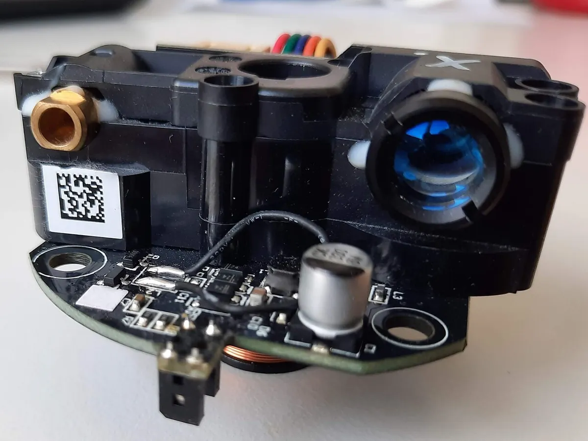
- Robot vacuums and warehouse robots: small spinning lidars give range readings that the robot must clean up and map.
- Drones: IMU noise and bias are simulated so the flight controller learns to cope before the first real flight.
- Your lab: a measured
<noise>block for each joint pot makes the Stage 12 digital twin behave like your desk arm.

Think
Think about it
Think
Your simulated range sensor returns the exact distance every 1 ms. Your real ultrasonic sensor returns a reading every 60 ms, with about 5 mm noise and occasional no-echo. Your stop-before-the-wall code worked perfectly in simulation. List three things that can go wrong on the real robot, and how you would change the simulated sensor to catch them first.
Experiment
Try it in the lab
About 60 minutes. Python 3 for the script; an Arduino UNO, a 10 kΩ pot and a push button for the bench.
Experiment
Measure the real sensor, then make the simulated one match
You will need
- `sensor_sim_lab.py` (Python 3, no libraries)
- Sensor simulation lab (in your browser)
- Arduino UNO, 10 kΩ potentiometer, push button, jumper wires
- Optional: a servo with its own 5–6 V supply to see supply noise
Steps
- Run `sensor_sim_lab.py` and note the gyro drift and the latency results.
- Bench: run `sensor_noise_meter.ino` three times with the knob still. Write down the stddev and step size.
- Copy your stddev (in degrees) into part 1 of the script as a noise term on the 10-bit pot reading. Does the reading still land on the truth?
- In part 4, change Kp to 8. What delay can it now tolerate? Check with π/(2·Kp).
- In part 2, subtract an estimated bias (average 2 s of readings while still) before integrating. How much drift is left after 60 s?
- In the sensor simulation lab, raise the noise to 5 and press “Resample noise” ten times. How much does the encoder reading jump?
Interactive · Sensor simulation lab · Educational
Reports joint angle from sim truth + optional noise. Educational — not a real AS5048 / magnetic encoder driver.
Sensor
Joint encoder
Reading
43.5°
Model
truth+noise
Educational sensor stubs — not ROS sensor_msgs, not Gazebo plugins, not live cameras/IMUs. Use noise & latency sliders to feel the sim-to-real gap.
The bench numbers are small but not zero, and they get worse when motors run. Bias removal kills most gyro drift. Lower gains tolerate more delay, at the cost of a slower move.
Knowledge check
Check your understanding
Knowledge check
1. Why add noise to a simulated sensor?
2. A 12-bit encoder over 360° has a step of about…
3. A gyro has a constant 0.005 rad/s bias. After integrating for 60 s, heading error is about…
4. Which SDF noise type adds rounding to Gaussian noise?
5. ROS `sensor_msgs/Imu` expects linear acceleration in…
6. Adding sensor delay to a fast P controller usually…
7. A lidar updates at 10 Hz on a robot moving at 0.5 m/s. Distance travelled between readings?
Mini assignment
Hands-on assignment
Mini assignment
A sensor card for your desk arm’s digital twin
Measure every sensor on your arm and write simulated-sensor settings that match.
Deliverables
- For each joint pot or encoder: measured stddev and step size (still and with servos running), and a `<noise type="gaussian_quantized">` block in radians.
- For one range sensor (ultrasonic or ToF): min and max range you measured, update rate, noise, and what the sensor returns when there is no target.
- A Python test that feeds your simulated sensors into the Lesson 7 PD controller and shows whether it still settles.
- A short note: which sensor effect hurt your controller most, and what you will change.
Do this, step by step
- Run
sensor_noise_meter.inowith the arm still, then with the servos running. - Work out the stddev and step size for each pot or encoder and convert to radians.
- Write a
<noise type="gaussian_quantized">block from your numbers. - Measure min range, max range, rate and the “no target” value for your range sensor.
- Feed your simulated sensors into the Lesson 7 PD controller with
sensor_sim_lab.pyand check it still settles.
Stuck? Hints, one at a time
- Noise with the servos running is often bigger, because of supply ripple. Use that number in the simulator.
- Step size (quantisation) is one ADC count turned into radians, not the stddev.
- If the controller wobbles only with noise, try a little less
kd: the derivative makes noise bigger.
Challenges (pick by level)
- 🟢 Beginner: Read your phone’s compass app while the phone lies still for a minute. Does the number wander? Write down how much.
- 🟡 Intermediate: Add a moving-average filter of 5 samples to the encoder in part 1. How much does the noise drop, and how much delay does it add?
- 🟠 Advanced: Add a slowly wandering bias (a random walk) to the gyro in part 2, like SDF’s dynamic bias. Show how a bias estimated at start stops working after a few minutes.
- 🔴 Expert: Build a simple complementary filter that mixes a noisy accelerometer tilt with a biased gyro rate. Compare its error with each sensor alone.
- ⚫ Research: Read the Gazebo sensors tutorial and the SDF noise element. Write one page on which sensor effects are hardest to simulate well (for example, ultrasonic echoes off soft or angled surfaces) and why.
Next step
The simulated robot can now feel the world like a real one. In Lesson 11 — Simulated Robot Controllers you will close the loop: controllers that read these simulated sensors and command the simulated joints, exactly the way they will on hardware.
Look back: Lesson 9: Friction & Physical Constraints. Next: Lesson 11: Simulated Robot Controllers. Related: Stage 11 — Computer Vision.
Sources
- Gazebo Harmonic — Sensors tutorial — IMU, contact and lidar sensors;
<update_rate>, lidar range 0.08–10 m at 10 Hz. - SDFormat 1.9 — noise element — types none/gaussian/gaussian_quantized; mean, stddev, bias_mean, bias_stddev, dynamic bias, precision.
- ROS 2 `sensor_msgs/Imu` message — m/s² and rad/s; covariance all zero means unknown.
- Photos: Wikimedia Commons (credits under each image).
Self-attested for now — keep artifacts in your lab notebook.
Complete
Today's goal
0 of 1 done today
Mark this lesson complete when you have worked the experiment, knowledge check, and assignment (even roughly).