
Robot Simulation & Digital Twin · Lesson 11
Simulated Robot Controllers
Est. 55–70 min
Why
Why this lesson matters
A simulator without a controller is only a movie: the arm falls under gravity and lies there. A controller closes the loop — read the sensor, decide a command, send it to the joint, repeat. In this lesson you will run that loop on a simulated joint, see how the command interface, the update rate and integral wind-up change the result, and then do a sim-to-real check with the noise and delay from Lesson 10.
On the bench you will run a tiny simulated joint *inside the Arduino* and tune its controller with two knobs and the Serial Plotter — a real-time digital twin on a low-cost board.
Concept
Closing the loop inside a simulator
1. The loop: read → update → write
Think of an auto-rickshaw driver keeping a steady speed on a flyover. He looks at the road (read), decides “a bit more throttle” (update), twists the grip (write), and does it again a moment later. ros2_control works the same way: its controller manager’s update() reads the hardware state, updates every active controller, and writes the commands back. In simulation, “hardware” is the simulated joint — for Gazebo, the gz_ros2_control plugin plays that role.
read()
get the latest joint position and velocity (state interfaces)
update()
each controller computes its command — for example PID on the error
write()
send the command to the joint (command interface) and hold it until the next cycle
physics steps
the simulator moves the joint for one or more physics steps
2. Command interfaces: what you are allowed to command
| Interface | You send | In simulation | Watch out |
|---|---|---|---|
| position | target angle | the simulator drives the joint towards it | can look perfect; hides motor strength |
| velocity | target speed | the joint is driven at that speed | gravity and torque limits partly hidden |
| effort | torque or force | the physics engine does all the rest | most honest; you must tune the controller |
<ros2_control name="GazeboSimSystem" type="system">
  <hardware>
    <plugin>gz_ros2_control/GazeboSimSystem</plugin>
  </hardware>
  <joint name="slider_to_cart">
    <command_interface name="effort">
      <param name="min">-1000</param>
      <param name="max">1000</param>
    </command_interface>
    <state_interface name="position">
      <param name="initial_value">1.0</param>
    </state_interface>
    <state_interface name="velocity"/>
    <state_interface name="effort"/>
  </joint>
</ros2_control>3. Three things that decide whether the controller works
- Update rate: a controller at 20 Hz acts on 50 ms-old information. Gains that are fine at 1000 Hz may oscillate.
- Saturation and wind-up: when the motor is at its torque limit, the integral term keeps growing and causes a big overshoot later. Anti-windup stops integrating while saturated.
- Sensor quality: noise makes the derivative term jumpy; delay reduces the stable gain range.
Visual
Visualise it: setpoint, command, joint, feedback
Robot controller simulator: position, velocity and effort modes on a toy joint, with live PID gains. (Educational plant, not ros2_control or Gazebo.)
Interactive · Robot controller simulator · Educational approximation

Educational browser plant only — not ros2_control, not Gazebo controller plugins, not real hardware. Mode switch mirrors position / velocity / effort interfaces conceptually (Stage 7 PID + Stage 10 msgs).
Code lab
Code lab: run a controller on a simulated joint
controller_sim_lab.py simulates one shoulder joint at 1 kHz with inertia, damping, gravity and a 0.4 N·m effort limit — the example numbers from Lessons 7–10. A PID controller runs the read → update → write loop at a rate you choose. Run python3 controller_sim_lab.py.
"""Simulated robot controllers lab (Stage 12, Lesson 11) - Python 3 standard library only.

One shoulder joint (example numbers from Lessons 7-10) is simulated at 1 kHz.
A controller runs the ros2_control-style loop:  read() -> update() -> write().

  1. Three command interfaces: position, velocity, effort (+PID)
  2. Controller update rate: the same PID at 1000, 200, 50 and 20 Hz
  3. Integral wind-up when the effort limit saturates, and a simple anti-windup
  4. Sim-to-real check: the same gains with sensor noise + 20 ms latency
All plant values are EXAMPLES - use your own arm's numbers.
"""
import math
import random

I, B, MGR = 0.005, 0.02, 0.20      # kg*m^2, N*m*s/rad damping, gravity torque m*g*r (N*m)
EFFORT_MAX, VEL_MAX = 0.4, 6.0     # N*m and rad/s (like URDF <limit>)
PHYS_DT = 0.001                    # physics step: 1 kHz
TARGET = 1.0                       # rad

def step_physics(q, w, tau):
    tau = max(-EFFORT_MAX, min(EFFORT_MAX, tau))
    alpha = (tau - B * w - MGR * math.sin(q)) / I
    w = max(-VEL_MAX, min(VEL_MAX, w + alpha * PHYS_DT))   # semi-implicit Euler (Lesson 6)
    return q + w * PHYS_DT, w, tau

def run(rate_hz=1000, kp=6.0, ki=2.0, kd=0.15, anti_windup=False, noise=0.0,
        latency_ms=0, t_end=2.0, seed=11):
    rng = random.Random(seed)
    q = w = integ = 0.0
    tau_cmd, prev_e = 0.0, TARGET
    every = max(1, int(round(1000 / rate_hz)))
    delay = int(latency_ms)                      # in physics steps (1 ms)
    seen = [0.0] * (delay + 1)
    peak, settle, sat_steps, late_err = 0.0, None, 0, 0.0
    for k in range(int(t_end / PHYS_DT)):
        seen.append(q + rng.gauss(0.0, noise) if noise else q)
        q_meas = seen.pop(0)                     # read(): late, noisy measurement
        if k % every == 0:                       # update(): only at the controller rate
            dt_c = every * PHYS_DT
            e = TARGET - q_meas
            d = (e - prev_e) / dt_c
            prev_e = e
            u = kp * e + ki * integ + kd * d
            saturated = abs(u) > EFFORT_MAX
            if not (anti_windup and saturated and (u * e) > 0):
                integ += e * dt_c                # stop integrating while pushing into the limit
            tau_cmd = u                          # write(): hold until next update
        q, w, tau_applied = step_physics(q, w, tau_cmd)
        if abs(tau_cmd) > EFFORT_MAX:
            sat_steps += 1
        peak = max(peak, q)
        if k * PHYS_DT >= t_end - 0.5:
            late_err = max(late_err, abs(q - TARGET))
        if abs(q - TARGET) > 0.02:
            settle = None
        elif settle is None:
            settle = k * PHYS_DT
    run.late_err = late_err
    return q, peak, settle, sat_steps * PHYS_DT

def fmt(q, peak, settle):
    s = f"settles {settle:.2f} s" if settle is not None else "NOT settled"
    return f"overshoot {max(0.0, peak - TARGET) / TARGET * 100:5.1f} %, {s}, final {math.degrees(q):6.1f} deg"

print(f"Joint: I {I} kg*m^2, damping {B}, gravity torque {MGR} N*m, effort limit {EFFORT_MAX} N*m")
print(f"Goal: 0 -> {TARGET} rad ({math.degrees(TARGET):.1f} deg)")
print()
print("=== 1. Command interfaces ===")
# position interface: the simulator moves the joint toward the target itself
q, gain, rate = 0.0, 0.1, 1000
for k in range(2000):
    vel = max(-VEL_MAX, min(VEL_MAX, gain * (TARGET - q) * rate))
    q += vel * PHYS_DT
    if k in (49, 199, 1999):
        print(f"  position  t {(k + 1) / 1000:4.2f} s: q {math.degrees(q):5.1f} deg  (simulator drives velocity = gain*error*rate)")
# velocity interface: P on position -> velocity command, motor torque not modelled
q = 0.0
for k in range(2000):
    vel = max(-VEL_MAX, min(VEL_MAX, 5.0 * (TARGET - q)))
    q += vel * PHYS_DT
    if k in (49, 199, 1999):
        print(f"  velocity  t {(k + 1) / 1000:4.2f} s: q {math.degrees(q):5.1f} deg  (P 5/s on position -> velocity command)")
print("  effort    PID on torque, with gravity and the 0.4 N*m limit:", fmt(*run()[:3]))
print("-> position/velocity interfaces in a simulator can look perfect because they ignore")
print("   how strong the motor is. The effort interface makes the controller fight real physics.")
print()
print("=== 2. Controller update rate (same PID gains kp 6, ki 2, kd 0.15) ===")
for hz in [1000, 200, 50, 20]:
    q, peak, settle, sat = run(rate_hz=hz)
    print(f"{hz:5d} Hz: {fmt(q, peak, settle)}")
print("-> slower loops act on older data; the derivative term becomes jumpy.")
print("   Tune in simulation at the SAME rate your real controller can run.")
print()
print("=== 3. Integral wind-up with a big step and strong integral (ki 8) ===")
for aw in [False, True]:
    q, peak, settle, sat = run(ki=8.0, anti_windup=aw, t_end=3.0)
    print(f"anti-windup {'ON ' if aw else 'OFF'}: {fmt(q, peak, settle)}, torque saturated for {sat:.2f} s")
print("-> while the motor is at its limit, the integral keeps growing; it must 'unwind' later.")
print()
print("=== 4. Sim-to-real check: same gains, 1 kHz, noise and latency added ===")
for label, noise, lat in [("perfect sensor", 0.0, 0),
                          ("noise 0.003 rad", 0.003, 0),
                          ("latency 20 ms", 0.0, 20),
                          ("noise + 20 ms", 0.003, 20)]:
    q, peak, settle, sat = run(noise=noise, latency_ms=lat, t_end=3.0)
    print(f"{label:>16}: overshoot {max(0.0, peak - TARGET) / TARGET * 100:5.1f} %, "
          f"worst error in the last 0.5 s {math.degrees(run.late_err):4.2f} deg")
print("-> if the controller only works with the perfect sensor, it is not ready for hardware.")
Output (run with python3 controller_sim_lab.py)
Joint: I 0.005 kg*m^2, damping 0.02, gravity torque 0.2 N*m, effort limit 0.4 N*m
Goal: 0 -> 1.0 rad (57.3 deg)

=== 1. Command interfaces ===
  position  t 0.05 s: q  17.2 deg  (simulator drives velocity = gain*error*rate)
  position  t 0.20 s: q  57.3 deg  (simulator drives velocity = gain*error*rate)
  position  t 2.00 s: q  57.3 deg  (simulator drives velocity = gain*error*rate)
  velocity  t 0.05 s: q  12.7 deg  (P 5/s on position -> velocity command)
  velocity  t 0.20 s: q  36.3 deg  (P 5/s on position -> velocity command)
  velocity  t 2.00 s: q  57.3 deg  (P 5/s on position -> velocity command)
  effort    PID on torque, with gravity and the 0.4 N*m limit: overshoot   6.7 %, settles 0.31 s, final   57.7 deg
-> position/velocity interfaces in a simulator can look perfect because they ignore
   how strong the motor is. The effort interface makes the controller fight real physics.

=== 2. Controller update rate (same PID gains kp 6, ki 2, kd 0.15) ===
 1000 Hz: overshoot   6.7 %, settles 0.31 s, final   57.7 deg
  200 Hz: overshoot   6.7 %, settles 0.30 s, final   57.7 deg
   50 Hz: overshoot  10.0 %, settles 0.71 s, final   57.8 deg
   20 Hz: overshoot  31.3 %, NOT settled, final   74.9 deg
-> slower loops act on older data; the derivative term becomes jumpy.
   Tune in simulation at the SAME rate your real controller can run.

=== 3. Integral wind-up with a big step and strong integral (ki 8) ===
anti-windup OFF: overshoot  18.8 %, settles 1.64 s, final   57.5 deg, torque saturated for 0.20 s
anti-windup ON : overshoot   3.1 %, settles 0.42 s, final   57.3 deg, torque saturated for 0.18 s
-> while the motor is at its limit, the integral keeps growing; it must 'unwind' later.

=== 4. Sim-to-real check: same gains, 1 kHz, noise and latency added ===
  perfect sensor: overshoot   6.7 %, worst error in the last 0.5 s 0.34 deg
 noise 0.003 rad: overshoot   9.9 %, worst error in the last 0.5 s 1.52 deg
   latency 20 ms: overshoot  16.8 %, worst error in the last 0.5 s 2.07 deg
   noise + 20 ms: overshoot  18.1 %, worst error in the last 0.5 s 1.79 deg
-> if the controller only works with the perfect sensor, it is not ready for hardware.
Try it: pick position, velocity or effort mode. In position mode move the setpoint and tune Kp, Ki, Kd; press Pause/Run and Reset. In effort mode the setpoint is a raw torque — watch the joint swing to its end. (Educational toy plant, not ros2_control.)
Interactive · Robot controller simulator · Educational approximation
Educational browser plant only — not ros2_control, not Gazebo controller plugins, not real hardware. Mode switch mirrors position / velocity / effort interfaces conceptually (Stage 7 PID + Stage 10 msgs).
Bench build: a digital twin joint inside the Arduino
servo_loop_rate.ino runs the same example joint at 1 kHz on the UNO, and a PID controller on top of it at a rate you set with a knob (10–500 Hz). A second knob sets the target angle; a button toggles anti-windup; an LED glows with the torque. Open the Serial Plotter to see target, angle and torque live.
| Part | Connection | Note |
|---|---|---|
| Pot 1 — target | outer legs 5V/GND, wiper A0 | 0–90° target |
| Pot 2 — controller rate | outer legs 5V/GND, wiper A1 | 10–500 Hz |
| Push button | D2 to GND | toggles anti-windup |
| LED + 220 Ω | D9 → resistor → LED → GND | brightness = |torque| / limit |
// servo_loop_rate.ino - Stage 12, Lesson 11: Simulated Robot Controllers
// A tiny "simulated joint" runs on the UNO at 1 kHz physics, and a PID controller
// runs on top of it at a rate YOU choose - just like a controller on a simulator.
//
// Wiring (no motors):
//   Pot 1 (target):  outer legs 5V/GND, wiper A0  -> target angle 0..90 deg
//   Pot 2 (rate):    outer legs 5V/GND, wiper A1  -> controller rate 10..500 Hz
//   Button D2 to GND (INPUT_PULLUP)               -> toggle anti-windup
//   LED + 220 ohm on D9 to GND                     -> brightness = |torque| / limit
// Open Serial Plotter at 115200 baud: target, angle and torque*100 are plotted.
// Same example joint as the Python lab: I 0.005, damping 0.02, gravity 0.2 N*m, limit 0.4 N*m.

const float I_J = 0.005, B_J = 0.02, MGR = 0.20, EFFORT_MAX = 0.4;
const float KP = 6.0, KI = 2.0, KD = 0.15;
const unsigned long PHYS_US = 1000;           // 1 kHz physics

float q = 0, w = 0, integ = 0, prevE = 0, tauCmd = 0;
bool antiWindup = false;
unsigned long lastPhys = 0, lastCtrl = 0, lastPrint = 0;

void setup() {
  Serial.begin(115200);
  pinMode(2, INPUT_PULLUP);
  pinMode(9, OUTPUT);
  lastPhys = micros();
  lastCtrl = lastPhys;
}

void loop() {
  unsigned long now = micros();

  // --- toggle anti-windup on button press ---
  static bool lastBtn = HIGH;
  bool btn = digitalRead(2);
  if (lastBtn == HIGH && btn == LOW) { antiWindup = !antiWindup; integ = 0; delay(20); }
  lastBtn = btn;

  float target = analogRead(A0) * (90.0 / 1023.0) * DEG_TO_RAD;
  int rateHz = map(analogRead(A1), 0, 1023, 10, 500);
  unsigned long ctrlUs = 1000000UL / rateHz;

  // --- controller: read() -> update() -> write() at the chosen rate ---
  if (now - lastCtrl >= ctrlUs) {
    float dt = (now - lastCtrl) / 1e6;
    lastCtrl = now;
    float e = target - q;                    // read(): our "sensor" is the simulated angle
    float d = (e - prevE) / dt;
    prevE = e;
    float u = KP * e + KI * integ + KD * d;  // update()
    bool sat = fabs(u) > EFFORT_MAX;
    if (!(antiWindup && sat && u * e > 0)) integ += e * dt;
    tauCmd = u;                              // write(): held until the next update
  }

  // --- physics at 1 kHz (semi-implicit Euler) ---
  while (now - lastPhys >= PHYS_US) {
    lastPhys += PHYS_US;
    float tau = constrain(tauCmd, -EFFORT_MAX, EFFORT_MAX);
    float alpha = (tau - B_J * w - MGR * sin(q)) / I_J;
    w += alpha * 0.001;
    q += w * 0.001;
    analogWrite(9, (int)(fabs(tau) / EFFORT_MAX * 255));
  }

  // --- plot at 25 Hz ---
  if (millis() - lastPrint >= 40) {
    lastPrint = millis();
    Serial.print(F("target:")); Serial.print(target * RAD_TO_DEG, 1);
    Serial.print(F(" angle:")); Serial.print(q * RAD_TO_DEG, 1);
    Serial.print(F(" torque_x100:")); Serial.print(constrain(tauCmd, -EFFORT_MAX, EFFORT_MAX) * 100, 1);
    Serial.print(F(" rate_hz:")); Serial.print(rateHz);
    Serial.print(F(" antiwindup:")); Serial.println(antiWindup ? 1 : 0);
  }
}Debugging
| Symptom | Likely cause | Fix |
|---|---|---|
| Perfect in simulation, shaky on hardware | position interface or perfect sensor in simulation | Use effort (or a realistic servo model) and add Lesson 10 noise and delay |
| Big overshoot after a long move | integral wind-up while saturated | Anti-windup or clamp the integral |
| Rings or oscillates at a low loop rate | gains tuned at a faster rate | Tune at the real rate; lower Kd/Kp |
| Joint chatters while holding still | noisy derivative | Filter the derivative or lower Kd |
| Joint sags below the target | gravity not overcome; no integral | Add Ki or gravity feed-forward (m·g·r·sin q) |
| Bench: plotter shows jagged lines | Serial printing too often | Keep printing at 25 Hz, as the sketch does |
Real world
Simulated controllers in the real world
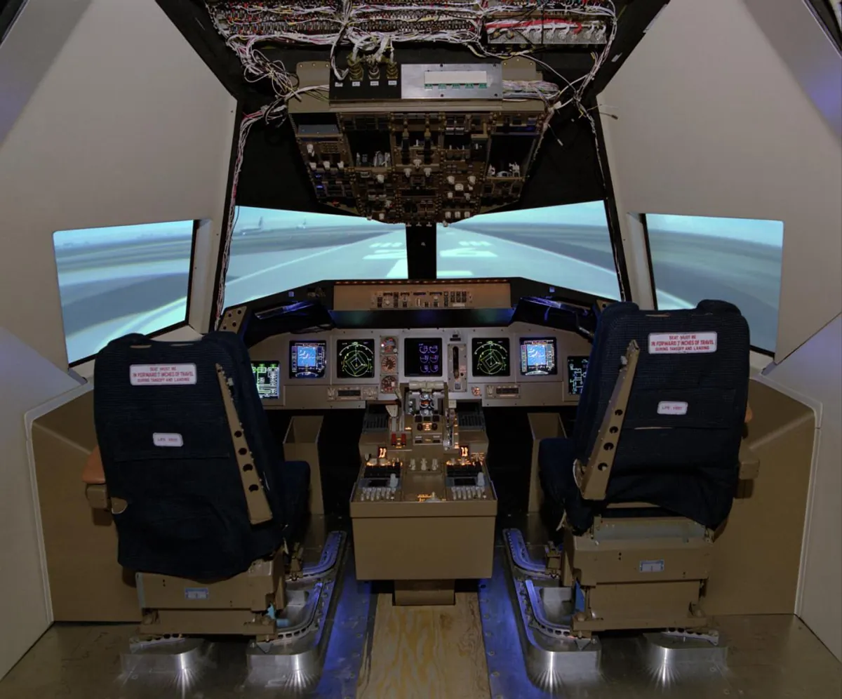
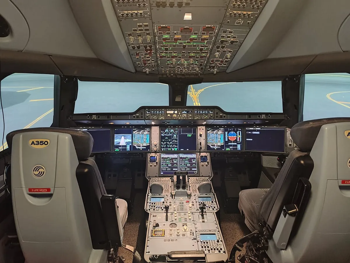
- Aviation: pilots and flight-control software are trained and tested in full-flight simulators before they fly.
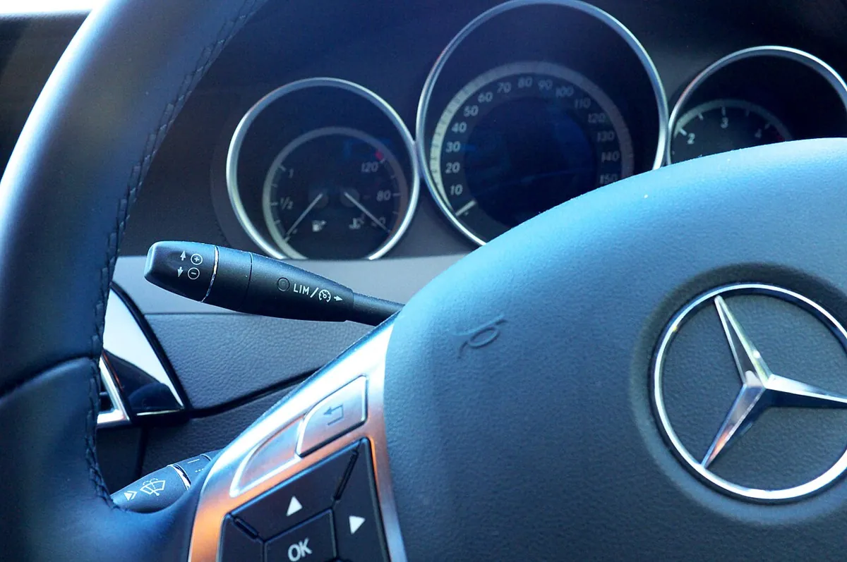
- Cars: cruise control and driver-assist controllers are tested on simulated roads and vehicles before road tests.
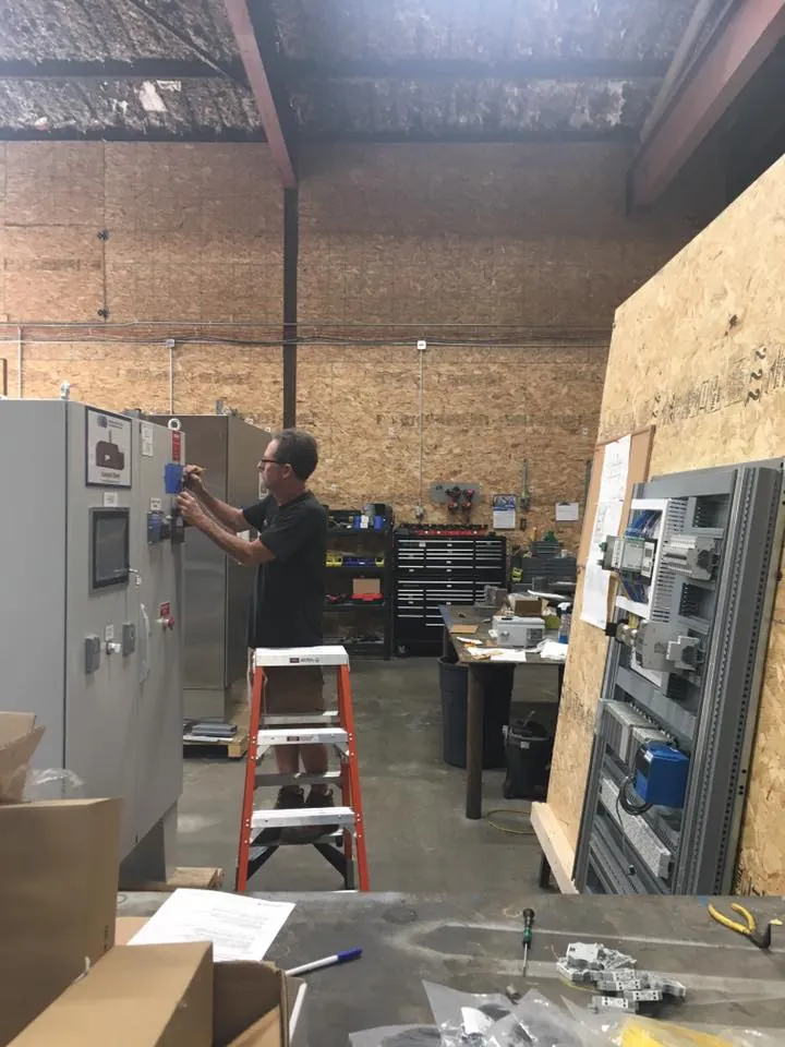
- Factories: PLC programs for machines are commonly checked against a virtual machine model (“virtual commissioning”) before the real machine is switched on.
- Robot arms: ros2_control lets the same controller configuration run against Gazebo or the real hardware by switching the hardware plugin.
Think
Think about it
Think
Your PID gains work beautifully in simulation at 1000 Hz with the position interface. Your real controller runs on an Arduino at 50 Hz and sends PWM to a hobby servo. List what is different, and how you would make the simulation closer before trusting the gains.
Experiment
Try it in the lab
About 60 minutes. Python 3 for the script; an Arduino UNO, two pots, a button, an LED and 220 Ω for the bench.
Experiment
Tune in simulation, then stress-test
You will need
- `controller_sim_lab.py` (Python 3, no libraries)
- Robot controller simulator (in your browser)
- Arduino UNO, two 10 kΩ pots, push button, LED + 220 Ω, jumper wires
Steps
- Run `controller_sim_lab.py`. Note the settle time at 1000 Hz and at 50 Hz.
- At 50 Hz, lower kd to 0.08 and kp to 4. Can you get it to settle within 0.6 s?
- Add gravity feed-forward: `u += MGR * math.sin(q_meas)` in `run()`. How do overshoot and settle time change?
- Turn on noise 0.003 and latency 20 ms with your new gains. Do they still work?
- Bench: on the Serial Plotter, find the lowest controller rate that still settles without ringing for a 0 → 60° step.
- In the browser simulator, set Kd to 0 in position mode and watch the overshoot; then raise it slowly.
Interactive · Robot controller simulator · Educational approximation
Educational browser plant only — not ros2_control, not Gazebo controller plugins, not real hardware. Mode switch mirrors position / velocity / effort interfaces conceptually (Stage 7 PID + Stage 10 msgs).
Gains are tied to the loop rate, the torque limit and the sensor quality. Gravity feed-forward lets the PID do less work. Good gains in an honest simulation need only a small trim on hardware.
Knowledge check
Check your understanding
Knowledge check
1. The three steps of the ros2_control loop are…
2. Which command interface makes the controller deal with real physics most honestly?
3. In gz_ros2_control the position interface’s velocity is…
4. Integral wind-up happens when…
5. Same PID gains, loop rate dropped from 1000 to 20 Hz. Most likely…
6. Why add sensor noise and delay before trusting simulated gains?
7. A simulated joint sags a little below its target and never quite reaches it. A good first fix?
Mini assignment
Hands-on assignment
Mini assignment
Tune one joint of your arm in simulation, then prove it
Use your arm’s real numbers to tune a shoulder controller in simulation and show it survives a sim-to-real stress test.
Deliverables
- Your joint’s inertia, gravity torque, damping guess and effort limit (from Lessons 7–9) in `controller_sim_lab.py`.
- Gains at your real controller rate that settle a 0 → 60° step in under 0.6 s with under 10 % overshoot.
- A table: perfect sensor vs your measured noise (Lesson 10) vs +20 ms delay — overshoot and final wobble for each.
- A Serial Plotter screenshot from `servo_loop_rate.ino` at your chosen rate, with and without anti-windup.
Do this, step by step
- Put your inertia, gravity torque, damping and effort limit into
controller_sim_lab.py. - Run a 0 → 60° step at your real controller rate.
- Tune gains until it settles in under 0.6 s with under 10 % overshoot.
- Run again with your noise from Lesson 10 and with +20 ms delay, and fill the table.
- Bench: run
servo_loop_rate.inoat your rate and take Serial Plotter shots with and without anti-windup.
Stuck? Hints, one at a time
- Change one gain at a time:
kpfor speed,kdfor overshoot,kionly for the last small error. TARGETis in radians: 60° is about 1.047 rad.- Without anti-windup the integral keeps growing while the motor is at its effort limit, which causes a big overshoot later.
Challenges (pick by level)
- 🟢 Beginner: In the browser simulator, find Kp/Ki/Kd values that reach 60° with almost no overshoot. Write them down.
- 🟡 Intermediate: Add a low-pass filter on the derivative in
run()and compare the noisy result with the plain derivative. - 🟠 Advanced: Model a hobby servo: a position command with a speed limit (for example 60° per 0.1 s) and a torque limit. Compare it with the effort PID.
- 🔴 Expert: Write a two-joint version (shoulder + elbow) with coupling — the elbow angle changes the shoulder’s gravity torque. Tune both loops.
- ⚫ Research: Read the ros2_control getting-started guide and gz_ros2_control docs. Explain how the same controller YAML can drive Gazebo and real hardware, and what has to change between them.
Next step
Your simulated controller works. In Lesson 12 — ROS 2 ↔ Simulator Communication you will connect it through ROS 2 topics — clock, joint states and commands — so the same nodes can talk to the simulator or the real arm.
Look back: Lesson 10: Simulated Sensors. Next: Lesson 12: ROS 2 ↔ Simulator Communication. Related: Stage 9 — Trajectory Planning.
Sources
- ros2_control — Getting started — the controller manager’s
update()reads hardware, updates active controllers, writes commands. - gz_ros2_control documentation (Jazzy) —
<ros2_control>tag with command/state interfaces,position_proportional_gain(default 0.1),hold_joints. - gz_ros2_control demo controller config —
update_rate: 1000, joint_trajectory_controller with position command interface. - Photos: Wikimedia Commons (credits under each image).
Self-attested for now — keep artifacts in your lab notebook.
Complete
Today's goal
0 of 1 done today
Mark this lesson complete when you have worked the experiment, knowledge check, and assignment (even roughly).