
Trajectory Planning & Motion Generation · Lesson 07
Cubic Polynomial Trajectories
Est. 50–70 min
Why
Why this lesson matters
In Lesson 1 you used the rest-to-rest cubic as a ready-made formula. In Lesson 6 you saw why plain lerp has corners. Now you will design cubics yourself. The idea is short and powerful: write the motion as q(t) = a0 + a1·t + a2·t² + a3·t³, list four conditions you want (positions and speeds at the start and end), and solve for the four coefficients. The same recipe gives you rest-to-rest moves, moves that end while still moving (for joining segments, as in Lesson 5), and the shortest time that respects your motor’s limits.
By the end of this lesson you will be able to: set up and solve the four equations of a cubic; use the closed-form coefficients from *Modern Robotics*; predict peak speed (1.5·d/T) and peak acceleration (6·d/T²) of a rest-to-rest cubic; compute the shortest feasible T from speed and acceleration limits; design a cubic with a non-zero end speed; explain the cubic’s one weakness — acceleration steps at the ends; and run a servo that refuses to move faster than its limits.
Concept
Four conditions, four coefficients
The cubic and its derivatives
position      q(t)  = a0 + a1·t + a2·t² + a3·t³
velocity      q̇(t)  = a1 + 2·a2·t + 3·a3·t²
acceleration  q̈(t)  = 2·a2 + 6·a3·t
jerk          q⃛(t)  = 6·a3          (constant)
Four unknowns need four conditions. For a move from q0 to qf in T seconds, the natural ones are: q(0) = q0, q̇(0) = v0, q(T) = qf, q̇(T) = vf. Putting t = 0 into the first two equations immediately gives a0 = q0 and a1 = v0. Putting t = T into the position and velocity equations gives two more equations for a2 and a3. *Modern Robotics* (Section 9.3, eq. 9.26–9.29) writes the result:
a0 = q0
a1 = v0
a2 = (3·qf − 3·q0 − 2·v0·T − vf·T) / T²
a3 = (2·q0 + (v0 + vf)·T − 2·qf) / T³
For the most common case — start and end at rest (v0 = vf = 0) and d = qf − q0 — this becomes a2 = 3d/T² and a3 = −2d/T³. That is exactly the Lesson 1 formula θ(t) = θstart + (3t²/T² − 2t³/T³)·d, which *Modern Robotics* derives in Section 9.2.2.
| Feature of the rest-to-rest cubic | Value | When |
|---|---|---|
| Peak speed | 1.5 · d / T | At t = T/2 |
| Peak acceleration | 6 · d / T² | At t = 0 (and −6·d/T² at t = T) |
| Shape of velocity | An upside-down parabola | Zero at both ends |
| Shape of acceleration | A straight line from +6d/T² to −6d/T² | Not zero at the ends |
Choosing T from the limits
Turn the two peak formulas around. If the joint must stay below a speed limit v_lim and an acceleration limit a_lim, then T must be at least 1.5·d / v_lim (speed) and at least √(6·d / a_lim) (acceleration). Take the larger of the two. Notice something interesting: for short moves the acceleration limit usually decides, for long moves the speed limit does. That is exactly what Part 3 of the code shows.
Visual
Visualise it: the cubic lab
Set q₀, q_f and T and scrub time: position, velocity and acceleration of a rest-to-rest cubic. Halve T and watch peak velocity double and peak acceleration go up four times.
Interactive · Cubic trajectory lab


Rest-to-rest cubic: q(0)=q₀, q(T)=q_f, q̇(0)=q̇(T)=0 → unique coefficients. Compare to linear lerp: cubic has continuous velocity (zero at ends) — kinder to motors and PID.
Position · q(t)
Velocity · q̇(t)
Acceleration · q̈(t)
q
34.6°
q̇
40.3°/s
q̈
13.4°/s²
Peak |q̇| scales ~1/T; peak |q̈| ~1/T². Shorten T → hotter motors / harder PID. Quintics (Part 2) also match acceleration at boundaries.
Code lab
Code lab: design, check and limit a cubic
cubic.py solves the four conditions as a 4×4 linear system (with its own small Gaussian elimination, so you can see every step), compares the answer with the closed-form coefficients, samples the motion, finds the shortest T for given limits, designs a cubic that ends while moving, and shows the acceleration step. Run python3 cubic.py.
"""cubic.py — Stage 9, Lesson 7
Design a cubic  q(t) = a0 + a1 t + a2 t^2 + a3 t^3  from FOUR conditions:
    q(0) = q0,  q'(0) = v0,  q(T) = qf,  q'(T) = vf
Part 1: solve the 4x4 system by hand-written Gaussian elimination and compare with the
        closed form (Modern Robotics eq. 9.26-9.29; rest-to-rest case eq. 9.11).
Part 2: sample the rest-to-rest cubic and check peak speed 1.5 d/T and peak accel 6 d/T^2.
Part 3: the shortest T that respects a speed AND an acceleration limit.
Part 4: a cubic that ends while still moving (vf != 0).
Part 5: the cubic's weak spot - acceleration jumps at the start and end.
"""
import math


def solve(A, b):
    """Gaussian elimination with partial pivoting (no numpy needed)."""
    n = len(b)
    M = [row[:] + [b[i]] for i, row in enumerate(A)]
    for c in range(n):
        p = max(range(c, n), key=lambda r: abs(M[r][c]))
        M[c], M[p] = M[p], M[c]
        for r in range(c + 1, n):
            f = M[r][c] / M[c][c]
            M[r] = [x - f * y for x, y in zip(M[r], M[c])]
    x = [0.0] * n
    for r in range(n - 1, -1, -1):
        x[r] = (M[r][n] - sum(M[r][k] * x[k] for k in range(r + 1, n))) / M[r][r]
    return x


def cubic_coeffs_matrix(q0, v0, qf, vf, T):
    A = [[1, 0, 0, 0],             # q(0)  = a0
         [0, 1, 0, 0],             # q'(0) = a1
         [1, T, T**2, T**3],       # q(T)
         [0, 1, 2*T, 3*T**2]]      # q'(T)
    return solve(A, [q0, v0, qf, vf])


def cubic_coeffs_closed(q0, v0, qf, vf, T):
    return [q0, v0,
            (3*qf - 3*q0 - 2*v0*T - vf*T) / T**2,
            (2*q0 + (v0 + vf)*T - 2*qf) / T**3]


def evaluate(c, t):
    return (c[0] + c[1]*t + c[2]*t**2 + c[3]*t**3,
            c[1] + 2*c[2]*t + 3*c[3]*t**2,
            2*c[2] + 6*c[3]*t)


Q0, QF, T = 30.0, 120.0, 1.5
cm = cubic_coeffs_matrix(Q0, 0, QF, 0, T)
cc = cubic_coeffs_closed(Q0, 0, QF, 0, T)
print("Part 1 - coefficients for 30 -> 120 deg in 1.5 s, starting and ending at rest")
print("  from the 4x4 solve :", [round(x, 4) for x in cm])
print("  from the formula   :", [round(x, 4) for x in cc])
print(f"  check: a2 = 3d/T^2 = {3*(QF-Q0)/T**2:.4f}, a3 = -2d/T^3 = {-2*(QF-Q0)/T**3:.4f}")

print("\nPart 2 - sampled every 0.25 s")
print("  t(s)    q(deg)   v(deg/s)   a(deg/s^2)")
for k in range(7):
    t = k * 0.25
    q, v, a = evaluate(cc, t)
    print(f"{t:5.2f}  {q:8.2f}  {v:8.2f}  {a:10.2f}")
d = QF - Q0
vs = [abs(evaluate(cc, T*n/1000)[1]) for n in range(1001)]
acs = [abs(evaluate(cc, T*n/1000)[2]) for n in range(1001)]
print(f"peak |v| {max(vs):.2f} (formula 1.5 d/T = {1.5*d/T:.2f}),  peak |a| {max(acs):.2f} (formula 6 d/T^2 = {6*d/T**2:.2f})")

print("\nPart 3 - shortest T for limits v <= 100 deg/s and a <= 200 deg/s^2")
VL, AL = 100.0, 200.0
for dd in (20.0, 90.0, 150.0):
    t_v = 1.5 * dd / VL
    t_a = math.sqrt(6 * dd / AL)
    Tmin = max(t_v, t_a)
    which = "speed" if t_v >= t_a else "acceleration"
    print(f"  move {dd:5.1f} deg: T from speed {t_v:.3f} s, from accel {t_a:.3f} s -> T_min = {Tmin:.3f} s ({which} limit decides)")

print("\nPart 4 - a cubic that keeps moving: 30 -> 120 deg in 1.5 s, ending at 40 deg/s")
c4 = cubic_coeffs_closed(30, 0, 120, 40, 1.5)
for t in (0.0, 0.75, 1.5):
    q, v, a = evaluate(c4, t)
    print(f"  t = {t:4.2f}  q = {q:7.2f}  v = {v:6.2f}  a = {a:8.2f}")

print("\nPart 5 - acceleration right before and right after the start of the rest-to-rest cubic")
print(f"  just before t = 0 (robot resting): 0.00 deg/s^2;  at t = 0+: {evaluate(cc, 0)[2]:.2f} deg/s^2")
print(f"  jerk q''' = 6*a3 = {6*cc[3]:.2f} deg/s^3 throughout, but the jump at t = 0 and t = T is a step -> infinite jerk")
print("  (Lesson 8's quintic adds two more conditions, a(0) = a(T) = 0, to remove these steps)")
Output (run with python3 cubic.py)
Part 1 - coefficients for 30 -> 120 deg in 1.5 s, starting and ending at rest
  from the 4x4 solve : [30.0, 0.0, 120.0, -53.3333]
  from the formula   : [30.0, 0, 120.0, -53.3333]
  check: a2 = 3d/T^2 = 120.0000, a3 = -2d/T^3 = -53.3333

Part 2 - sampled every 0.25 s
  t(s)    q(deg)   v(deg/s)   a(deg/s^2)
 0.00     30.00      0.00      240.00
 0.25     36.67     50.00      160.00
 0.50     53.33     80.00       80.00
 0.75     75.00     90.00        0.00
 1.00     96.67     80.00      -80.00
 1.25    113.33     50.00     -160.00
 1.50    120.00      0.00     -240.00
peak |v| 90.00 (formula 1.5 d/T = 90.00),  peak |a| 240.00 (formula 6 d/T^2 = 240.00)

Part 3 - shortest T for limits v <= 100 deg/s and a <= 200 deg/s^2
  move  20.0 deg: T from speed 0.300 s, from accel 0.775 s -> T_min = 0.775 s (acceleration limit decides)
  move  90.0 deg: T from speed 1.350 s, from accel 1.643 s -> T_min = 1.643 s (acceleration limit decides)
  move 150.0 deg: T from speed 2.250 s, from accel 2.121 s -> T_min = 2.250 s (speed limit decides)

Part 4 - a cubic that keeps moving: 30 -> 120 deg in 1.5 s, ending at 40 deg/s
  t = 0.00  q =   30.00  v =   0.00  a =   186.67
  t = 0.75  q =   67.50  v =  80.00  a =    26.67
  t = 1.50  q =  120.00  v =  40.00  a =  -133.33

Part 5 - acceleration right before and right after the start of the rest-to-rest cubic
  just before t = 0 (robot resting): 0.00 deg/s^2;  at t = 0+: 240.00 deg/s^2
  jerk q''' = 6*a3 = -320.00 deg/s^3 throughout, but the jump at t = 0 and t = T is a step -> infinite jerk
  (Lesson 8's quintic adds two more conditions, a(0) = a(T) = 0, to remove these steps)
Try it: compare cubic with linear and quintic. Look closely at the acceleration plot at t = 0 and t = T — the cubic starts and ends with a jump.
Interactive · Motion profile comparator


Overlay linear, cubic, and quintic rest-to-rest profiles. Linear has velocity steps (harsh); cubic zeros velocity; quintic also zeros acceleration — lowest jerk among the three.
Position q(t)
Velocity q̇(t)
Acceleration q̈(t)
Jerk q⃛(t)
| Profile | peak |q̇| | peak |q̈| | peak |jerk| |
|---|---|---|---|
| Linear | 36.0 | 0.0 | ∞ (edge) |
| Cubic | 54.0 | 86.4 | 69.1 |
| Quintic | 67.5 | 83.1 | 345.6 |
Educational 1-DOF overlays — not full multi-DOF dynamics. Linear jerk shown as edge impulse in table.
Real world
Cubic motion in the real world
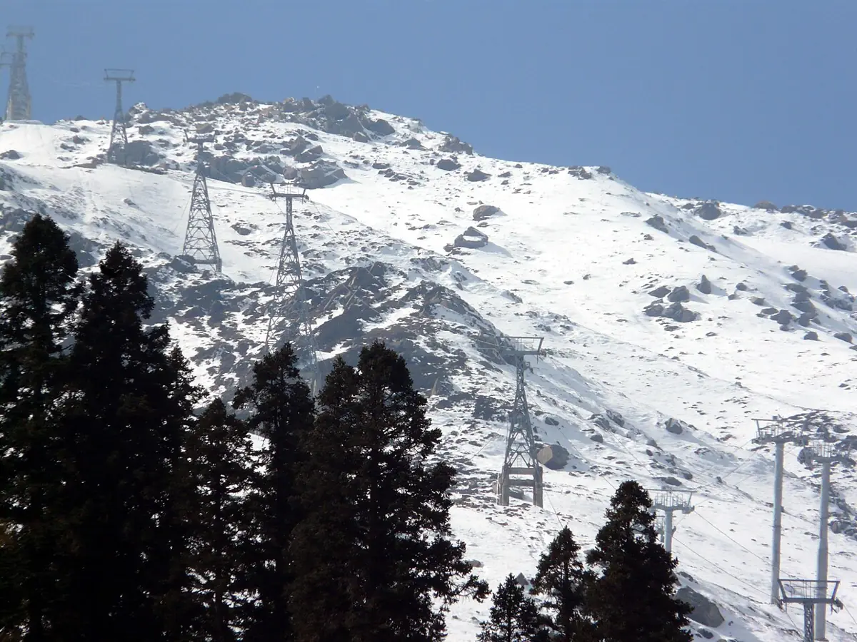
- Ropeways and lifts: cabins and cars leave and arrive at rest; their drives shape speed so passengers are not thrown about.
- Robot joint moves: many simple controllers use polynomial time scalings for point-to-point joint moves, because they are cheap to compute on a small processor — just a few multiplications per step.
- Camera sliders and pan-tilt heads: “ease in, ease out” settings are smooth polynomials so the shot starts and stops without a jolt.
- Animation: key-frame tools interpolate between poses with cubic curves so characters move naturally.

Bench build
Bench build: a servo that respects its limits
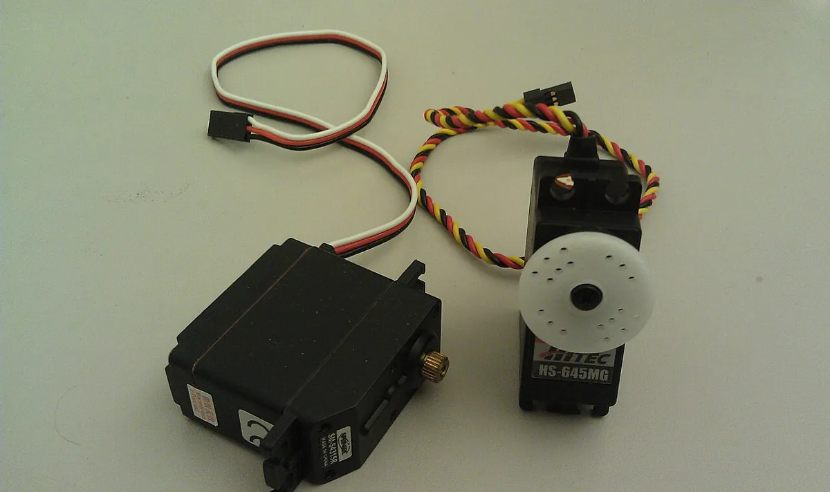
One servo with a stick arm, as in Lesson 1. cubic_servo.ino waits for a command like 120 1.5 in the Serial Monitor (“move to 120° in 1.5 s”). It computes the peak speed and acceleration of that cubic, compares them with the limits you set (100°/s and 200°/s² by default), stretches T if needed and tells you so, then runs the move.
| From | To | Note |
|---|---|---|
| Servo signal | D9 | — |
| Servo + and − | Separate 5–6 V supply | Never the Arduino 5 V pin |
| Supply − | Arduino GND | Common ground |
Open the Serial Monitor
115200 baud, line ending “Newline”. The servo sits at 90°.
A reasonable move
Type
120 1.5. 30° in 1.5 s is well within limits: it runs as asked.A move that is too fast
Type
30 0.5. 90° in 0.5 s would need 270°/s and 2160°/s². The sketch stretches T to about 1.64 s and prints why.Out of range
Type
175 2. It is refused: the sketch keeps the servo inside 10°–170° to stay off its end stops.Your limits
Lower V_LIM to 60 and A_LIM to 100, upload, and repeat. Which moves get stretched now?
// cubic_servo.ino — Stage 9, Lesson 7
// Type a target in the Serial Monitor (115200, "Newline"):   <angle> <seconds>
//   e.g.  120 1.5
// The sketch designs a rest-to-rest cubic from the current angle, checks it against
// speed and acceleration limits, STRETCHES T if needed (and tells you), then runs it.
//   peak speed = 1.5*d/T,  peak acceleration = 6*d/T^2   (Modern Robotics 9.2.2.1)
// Wiring: servo signal -> D9; servo + and - -> SEPARATE 5–6 V supply; supply GND -> Arduino GND.
// Never power the servo from an Arduino pin.

#include <Servo.h>

const float V_LIM = 100.0;      // deg/s   (example limits — choose safe values for your servo)
const float A_LIM = 200.0;      // deg/s^2
const float MIN_DEG = 10.0, MAX_DEG = 170.0;   // keep away from end stops
const unsigned long DT_MS = 20;

Servo s;
float current = 90.0;

void writeDeg(float d) {
  s.writeMicroseconds(544 + (long)(d * (2400 - 544) / 180.0 + 0.5));
}

void runCubic(float q0, float qf, float T) {
  float d = qf - q0;
  float a2 = 3.0 * d / (T * T), a3 = -2.0 * d / (T * T * T);
  unsigned long t0 = millis(), next = t0;
  while (true) {
    unsigned long now = millis();
    if (now < next) continue;
    next += DT_MS;
    float t = (now - t0) / 1000.0;
    if (t > T) t = T;
    float q = q0 + a2 * t * t + a3 * t * t * t;
    writeDeg(q);
    if (t >= T) break;
  }
  current = qf;
}

void setup() {
  Serial.begin(115200);
  s.attach(9);
  writeDeg(current);
  Serial.println(F("Type: <angle> <seconds>   e.g. 120 1.5"));
}

void loop() {
  if (!Serial.available()) return;
  float goal = Serial.parseFloat();
  float T = Serial.parseFloat();
  while (Serial.available()) Serial.read();        // clear the rest of the line
  if (goal < MIN_DEG || goal > MAX_DEG) { Serial.println(F("REFUSED: angle outside 10..170")); return; }
  if (T <= 0) T = 1.0;

  float d = fabs(goal - current);
  float tV = 1.5 * d / V_LIM;
  float tA = sqrt(6.0 * d / A_LIM);
  float tMin = max(tV, tA);
  Serial.print(F("move ")); Serial.print(d, 1); Serial.print(F(" deg, asked T = ")); Serial.print(T, 2);
  Serial.print(F(" s, peak v ")); Serial.print(1.5 * d / T, 1);
  Serial.print(F(", peak a ")); Serial.println(6.0 * d / (T * T), 1);
  if (T < tMin) {
    Serial.print(F("  too fast -> stretched to T = ")); Serial.print(tMin, 2); Serial.println(F(" s"));
    T = tMin;
  }
  runCubic(current, goal, T);
  Serial.println(F("  done"));
}
Debugging
Debugging cubic trajectories
| Symptom | Likely cause | Fix |
|---|---|---|
| Move overshoots the goal and comes back | Non-zero end velocity with too short T, or wrong sign of a3 | Recheck a2, a3; plot q(t) |
| Arm ends at the wrong angle | t not clamped to T at the end | Clamp t, and write the exact goal at the end |
| Peak speed is twice what you computed | Used d/T instead of 1.5·d/T, or T in ms | Use seconds and the 1.5 factor |
| T_min seems too long for short moves | Acceleration limit decides for short moves | Expected — √(6d/a_lim) dominates |
| A small “kick” at start and end | Cubic acceleration step | Use a quintic (Lesson 8) for delicate loads |
Think
Think about it
Think
You must move a joint 90° and your limits are 100°/s and 200°/s². A friend says, “Just double the speed limit and the move will take half the time.” Use Part 3 of the output to check whether that is true.
Experiment
Try it in the lab
About 35 minutes with cubic.py, the browser labs and (optionally) the servo.
Experiment
Design your own cubics
You will need
- `cubic.py` and Python 3
- Graph paper or a spreadsheet
- Cubic trajectory lab and motion profile comparator (in your browser)
- Optional: Arduino UNO, one servo, separate 5–6 V supply
Steps
- Run `cubic.py`. Plot q, v and a from Part 2 on three stacked graphs.
- Change T to 0.75 s. Predict the new peak speed and acceleration before running. Check.
- In Part 3, find the move size at which the speed and acceleration limits give the same T (hint: set 1.5d/V = √(6d/A) and solve for d).
- In Part 4, try vf = 120°/s. Does the position overshoot 120° before the end? Plot it.
- Add a case to Part 1 with v0 = 20, vf = −20. Check the matrix solve still matches the formula.
- Optional: on the bench, find the smallest T the sketch accepts for a 60° move without stretching.
Interactive · Cubic trajectory lab
Rest-to-rest cubic: q(0)=q₀, q(T)=q_f, q̇(0)=q̇(T)=0 → unique coefficients. Compare to linear lerp: cubic has continuous velocity (zero at ends) — kinder to motors and PID.
Position · q(t)
Velocity · q̇(t)
Acceleration · q̈(t)
q
34.6°
q̇
40.3°/s
q̈
13.4°/s²
Peak |q̇| scales ~1/T; peak |q̈| ~1/T². Shorten T → hotter motors / harder PID. Quintics (Part 2) also match acceleration at boundaries.
Four conditions fix a cubic completely. Rest-to-rest cubics have peak speed 1.5d/T at mid-time and peak acceleration 6d/T² at the ends. Short moves are acceleration-limited, long ones speed-limited. Non-zero end speeds let segments join smoothly, but large ones can cause overshoot. Acceleration still jumps at the ends.
Knowledge check
Check your understanding
Knowledge check
1. How many conditions are needed to fix a cubic trajectory?
2. For any cubic, a0 and a1 equal…
3. A rest-to-rest cubic moves 60° in 2 s. Its peak speed is…
4. Same move (60° in 2 s). Peak acceleration is…
5. Limits 100°/s and 200°/s². For a 20° move, which limit decides T?
6. What is the main weakness of the rest-to-rest cubic?
7. Why would you design a cubic with a non-zero end velocity?
Mini assignment
Hands-on assignment
Mini assignment
A cubic planner for your arm
Write a reusable cubic planner, choose safe limits for one joint of your arm, and prove each move is feasible before it runs.
Deliverables
- Function `plan_cubic(q0, qf, v0, vf, T)` returning the coefficients, and `t_min(d, v_lim, a_lim)` for rest-to-rest moves.
- A table of 5 moves for one joint of your arm (your own angles), each with T_min, which limit decides, and the peak values at that T.
- Plots of q, v, a for your largest move.
- Run two of your moves on the servo with `cubic_servo.ino` (your own limits) and note whether any were stretched.
- Two sentences: why short moves are acceleration-limited and long moves speed-limited.
Do this, step by step
- Run
python3 cubic.pyand check that Part 1 (matrix) and the closed-form coefficients match. - In Part 3, write the shortest T for the example move and which limit (speed or acceleration) decides it.
- Write
t_min(d, v_lim, a_lim)= max(1.5·d/v_lim, √(6·d/a_lim)) and test it on a 10° move and a 120° move. Which limit wins for each? - Read Part 5 and write what happens to acceleration at t = 0 and t = T.
- Optional bench: in
cubic_servo.ino, setV_LIMandA_LIMto your joint’s values and run two of your moves. Note any that were stretched.
Stuck? Hints, one at a time
- A cubic has 4 coefficients, so it can meet 4 conditions: start and end position, start and end speed.
- Short moves are acceleration-limited (T grows like √d); long moves are speed-limited (T grows like d).
- The cubic’s acceleration does not start at zero — that jump is the weak spot the quintic fixes in Lesson 8.
Challenges (pick by level)
- 🟢 Easy: Compute a2 and a3 by hand for 0° → 90° in 3 s, rest to rest.
- 🟢 Easy: For that move, find the time when the joint is exactly at 45°. (Hint: by symmetry.)
- 🟡 Medium: Make
cubic.pyprint a text plot of the velocity curve (like Lesson 3, Part 4). - 🟠 Hard-ish: Chain three cubics through waypoints 0° → 60° → 90° → 30° with sensible via velocities, and check continuity at each join.
- 🔴 Hard: Run two joints with different move sizes but the same T so they start and finish together (a first taste of Lesson 14 synchronisation). Which joint decides T?
- ⚫ Research: Read *Modern Robotics* §9.2.2.1 and explain why the book says the cubic leads to infinite jerk at the start and end.
Next step
You have now finished the joint-space foundations of this stage. Next, Lesson 8 — Quintic Polynomial Trajectories adds two more wishes — zero acceleration at both ends — to remove the cubic’s last jolt.
Look back: Lesson 6: Linear Interpolation. Next: Lesson 8: Quintic Polynomial Trajectories. Related: Stage 7 — Control Systems & PID.
Sources
- Modern Robotics (Lynch & Park) — book home page and free PDF — §9.2.2.1 third-order time scaling (a2 = 3/T², a3 = −2/T³; peak velocity 3/(2T)·d at T/2; peak acceleration 6/T²·d; checking or solving T from limits; infinite jerk at the ends); §9.3 cubic via-point coefficients eq. 9.26–9.29.
- Modern Robotics video — 9.1 and 9.2 Point-to-Point Trajectories — companion lecture.
- Wikipedia — Jerk (physics) — jerk as the rate of change of acceleration.
- Arduino — Servo library —
writeMicroseconds()used to stream cubic set-points. - Photos: Wikimedia Commons (credits under each image).
Self-attested for now — keep artifacts in your lab notebook.
Complete
Today's goal
0 of 1 done today
Mark this lesson complete when you have worked the experiment, knowledge check, and assignment (even roughly).