
Trajectory Planning & Motion Generation · Lesson 03
Position, Velocity & Acceleration
Est. 45–60 min
Why
Why this lesson matters
In Lesson 1 you saw that a jump asks for impossible speed and acceleration. To design better motions you must be fluent in reading three curves together: position (where), velocity (how fast, and which way) and acceleration (how quickly the speed changes). Every motor has a limit on each one, every motion profile in this stage is judged by them, and every robot controller you meet — from a hobby servo board to an industrial robot — talks in these terms.
By the end of this lesson you will be able to: explain position, velocity, acceleration (and jerk) as rates of change; read a trapezoidal velocity profile phase by phase; get velocity and acceleration from position samples with finite differences; see why derivatives amplify sensor noise and how a small filter helps; and watch your own hand motion as three live curves on the Arduino Serial Plotter.
Concept
Three curves, one motion
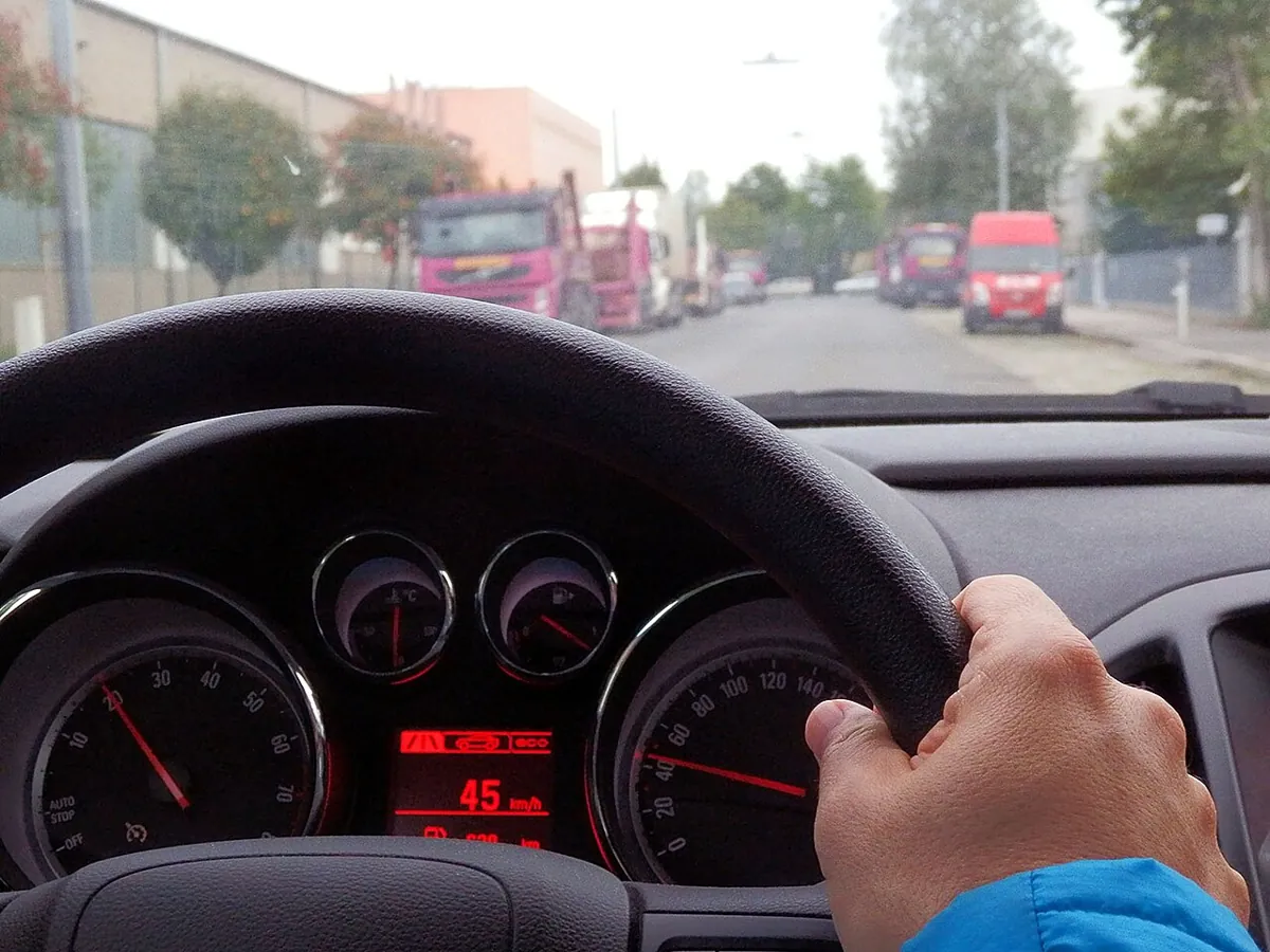
Each one is the rate of change of the one before
| Quantity | Symbol | Meaning | Unit for a joint | Scooter example |
|---|---|---|---|---|
| Position | θ | Where the joint is | ° (or rad) | Distance from home: 1.2 km |
| Velocity | θ̇ = dθ/dt | How fast position changes (with sign = direction) | °/s | 40 km/h on the speedometer |
| Acceleration | θ̈ = dθ̇/dt | How fast velocity changes | °/s² | Hard braking at the signal |
| Jerk | dθ̈/dt | How fast acceleration changes | °/s³ | The sudden “kick” when brakes bite |
Going down the table you differentiate (take the slope). Going up, you integrate (add up the area). So: the slope of the position curve at any moment is the velocity; the area under the velocity curve is the distance moved. If you remember just that one picture — slope going down, area going up — you can read any motion plot.
Reading a trapezoidal velocity profile
The most common profile in motor control is the trapezoid, named after the shape of its velocity curve. *Modern Robotics* (Section 9.2.2) describes it as three phases: constant acceleration, constant velocity (cruise) and constant deceleration. Our example joint moves 0° → 90° with cruise speed 60°/s and acceleration 120°/s²:
| Phase | Time | Position | Velocity | Acceleration |
|---|---|---|---|---|
| Speed up | 0 → 0.5 s | 0° → 15° (curving up, a parabola) | 0 → 60°/s (straight ramp) | +120°/s² (flat) |
| Cruise | 0.5 → 1.5 s | 15° → 75° (straight line) | 60°/s (flat) | 0 |
| Slow down | 1.5 → 2.0 s | 75° → 90° (curving flat) | 60 → 0°/s (ramp down) | −120°/s² (flat) |
time to reach cruise   ta = V / A            = 60 / 120 = 0.5 s
angle while speeding   da = ½ · A · ta²       = 15°
cruise angle           = D − 2·da             = 60°  → cruise time 60 / 60 = 1 s
total time T = 2·ta + cruise time = 2.0 sFrom samples to derivatives: finite differences
A robot never sees a smooth formula; it sees samples, for example an encoder reading every 20 ms. To estimate velocity, divide the change in position by the time step: v ≈ (θₖ − θₖ₋₁) / Δt. Do the same to velocities to get acceleration. This works beautifully on clean numbers — but every tiny measurement error is also divided by a small Δt, so noise gets multiplied. Differentiate twice and it gets multiplied again.
Visual
Visualise it: position, velocity and acceleration together
Change the start, goal and duration of a smooth move and watch the position, velocity and acceleration curves change together. Shorter T: taller velocity and much taller acceleration.
Interactive · Cubic trajectory lab


Rest-to-rest cubic: q(0)=q₀, q(T)=q_f, q̇(0)=q̇(T)=0 → unique coefficients. Compare to linear lerp: cubic has continuous velocity (zero at ends) — kinder to motors and PID.
Position · q(t)
Velocity · q̇(t)
Acceleration · q̈(t)
q
34.6°
q̇
40.3°/s
q̈
13.4°/s²
Peak |q̇| scales ~1/T; peak |q̈| ~1/T². Shorten T → hotter motors / harder PID. Quintics (Part 2) also match acceleration at boundaries.
Code lab
Code lab: build and read a PVA table
pva.py computes the exact trapezoid, then pretends it only has position samples (50 Hz) and recovers velocity and acceleration with finite differences. Then it adds ±0.5° of sensor noise to show what happens, and fixes it with a moving average. Run python3 pva.py.
"""pva.py — Stage 9, Lesson 3
Position, velocity and acceleration of ONE joint during a lift-style move.
Profile: trapezoidal velocity (Modern Robotics 9.2.2.2): speed up at constant
acceleration, cruise at constant speed, slow down at constant deceleration.
  move 0 -> 90 deg, cruise speed V = 60 deg/s, acceleration A = 120 deg/s^2 (example values)
"""
import random

D, V, A = 90.0, 60.0, 120.0
TA = V / A                      # time to reach cruise speed
DA = 0.5 * A * TA**2            # angle covered while speeding up
TV = (D - 2 * DA) / V           # cruise time
T = 2 * TA + TV                 # total time


def pva(t):
    """Exact position, velocity, acceleration of the trapezoid at time t."""
    if t <= 0:
        return 0.0, 0.0, 0.0
    if t < TA:                                   # speeding up
        return 0.5 * A * t**2, A * t, A
    if t < TA + TV:                              # cruising
        return DA + V * (t - TA), V, 0.0
    if t < T:                                    # slowing down
        r = T - t
        return D - 0.5 * A * r**2, A * r, -A
    return D, 0.0, 0.0


print(f"Part 1 - the plan: speed-up {TA:.2f} s ({DA:.0f} deg), cruise {TV:.2f} s ({V*TV:.0f} deg), slow-down {TA:.2f} s; total T = {T:.2f} s")
print("  t(s)   pos(deg)  vel(deg/s)  acc(deg/s^2)  phase")
for i in range(0, 10):
    t = i * 0.25
    p, v, a = pva(t)
    phase = "rest" if t == 0 or t >= T else ("speed-up" if t < TA else ("cruise" if t < TA + TV else "slow-down"))
    print(f"{t:5.2f}  {p:8.2f}  {v:9.1f}  {a:11.1f}    {phase}")

DT = 0.02                                        # 50 Hz samples, like a control loop
ts = [k * DT for k in range(int(T / DT) + 6)]
pos = [pva(t)[0] for t in ts]
vel = [(pos[k] - pos[k - 1]) / DT for k in range(1, len(pos))]
acc = [(vel[k] - vel[k - 1]) / DT for k in range(1, len(vel))]
print("\nPart 2 - recover velocity and acceleration from positions only (finite differences, 50 Hz)")
print(f"max |vel| from differences: {max(map(abs, vel)):6.1f} deg/s   (plan: {V:.1f})")
print(f"max |acc| from differences: {max(map(abs, acc)):6.1f} deg/s^2 (plan: {A:.1f})")
print(f"distance = area under velocity curve: {sum(v * DT for v in vel):.2f} deg (plan: {D:.0f})")

random.seed(7)
noisy = [p + random.uniform(-0.5, 0.5) for p in pos]   # sensor noise of +/-0.5 deg
nvel = [(noisy[k] - noisy[k - 1]) / DT for k in range(1, len(noisy))]
nacc = [(nvel[k] - nvel[k - 1]) / DT for k in range(1, len(nvel))]
cruise = [k for k, t in enumerate(ts[1:]) if TA + 0.1 < t < TA + TV - 0.1]
err_v = max(abs(nvel[k] - V) for k in cruise)
print("\nPart 3 - same thing with +/-0.5 deg sensor noise")
print(f"worst velocity error while cruising: {err_v:6.1f} deg/s")
print(f"max |acc| now: {max(map(abs, nacc)):8.1f} deg/s^2  <- noise is amplified by every derivative")

W = 5                                            # moving average over 5 samples (0.1 s)
sm = [sum(noisy[k - W + 1:k + 1]) / W for k in range(W - 1, len(noisy))]
svel = [(sm[k] - sm[k - 1]) / DT for k in range(1, len(sm))]
cr2 = [k for k in range(len(svel)) if TA + 0.2 < (k + W) * DT < TA + TV - 0.1]
print(f"after a 5-sample moving average, worst cruise velocity error: {max(abs(svel[k] - V) for k in cr2):5.1f} deg/s")

print("\nPart 4 - velocity as a text plot (one # = 4 deg/s)")
for i in range(0, 11):
    t = i * 0.2
    v = pva(t)[1]
    print(f"{t:4.1f}s |" + "#" * int(round(v / 4)))
Output (run with python3 pva.py)
Part 1 - the plan: speed-up 0.50 s (15 deg), cruise 1.00 s (60 deg), slow-down 0.50 s; total T = 2.00 s
  t(s)   pos(deg)  vel(deg/s)  acc(deg/s^2)  phase
 0.00      0.00        0.0          0.0    rest
 0.25      3.75       30.0        120.0    speed-up
 0.50     15.00       60.0          0.0    cruise
 0.75     30.00       60.0          0.0    cruise
 1.00     45.00       60.0          0.0    cruise
 1.25     60.00       60.0          0.0    cruise
 1.50     75.00       60.0       -120.0    slow-down
 1.75     86.25       30.0       -120.0    slow-down
 2.00     90.00        0.0          0.0    rest
 2.25     90.00        0.0          0.0    rest

Part 2 - recover velocity and acceleration from positions only (finite differences, 50 Hz)
max |vel| from differences:   60.0 deg/s   (plan: 60.0)
max |acc| from differences:  120.0 deg/s^2 (plan: 120.0)
distance = area under velocity curve: 90.00 deg (plan: 90)

Part 3 - same thing with +/-0.5 deg sensor noise
worst velocity error while cruising:   43.1 deg/s
max |acc| now:   4473.9 deg/s^2  <- noise is amplified by every derivative
after a 5-sample moving average, worst cruise velocity error:   5.3 deg/s

Part 4 - velocity as a text plot (one # = 4 deg/s)
 0.0s |
 0.2s |######
 0.4s |############
 0.6s |###############
 0.8s |###############
 1.0s |###############
 1.2s |###############
 1.4s |###############
 1.6s |############
 1.8s |######
 2.0s |
Try it: compare position, velocity and acceleration for linear, cubic and quintic profiles. Which one has jumps in velocity? Which one in acceleration?
Interactive · Motion profile comparator


Overlay linear, cubic, and quintic rest-to-rest profiles. Linear has velocity steps (harsh); cubic zeros velocity; quintic also zeros acceleration — lowest jerk among the three.
Position q(t)
Velocity q̇(t)
Acceleration q̈(t)
Jerk q⃛(t)
| Profile | peak |q̇| | peak |q̈| | peak |jerk| |
|---|---|---|---|
| Linear | 36.0 | 0.0 | ∞ (edge) |
| Cubic | 54.0 | 86.4 | 69.1 |
| Quintic | 67.5 | 83.1 | 345.6 |
Educational 1-DOF overlays — not full multi-DOF dynamics. Linear jerk shown as edge impulse in table.
Real world
PVA in the real world
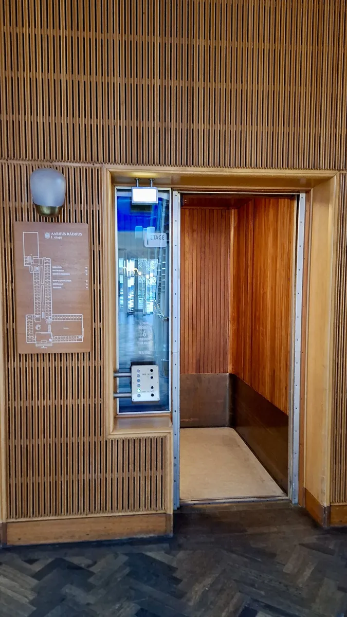
- Lifts (elevators): passengers feel acceleration and jerk, not speed. Lift drives limit both so a ride feels smooth even at high speed.
- Cars and bikes: the speedometer shows velocity; “0 to 100 km/h in 10 s” is an average acceleration statement.
- CNC machines and 3D printers: firmware such as Marlin has separate commands to set the maximum feedrate (velocity) and maximum acceleration of each axis (M203 and M201).
- Robot controllers: joint limits are written as maximum position range, velocity and acceleration — exactly the three quantities in this lesson.
Bench build
Bench build: see PVA of your own hand
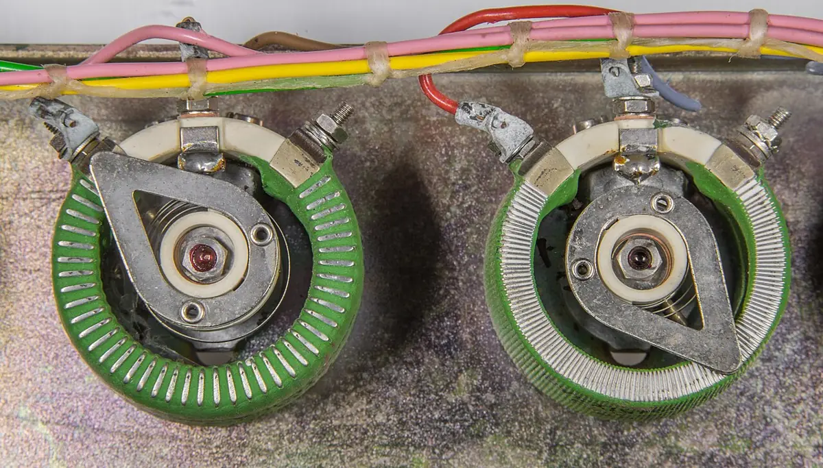
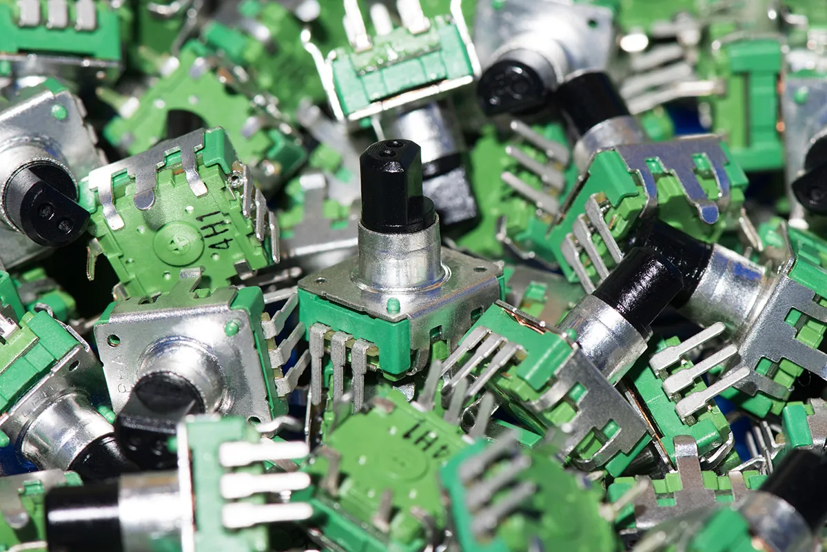
One 10 kΩ potentiometer is your “joint”. pva_knob.ino samples it at exactly 50 Hz, filters it, and prints position, velocity and acceleration (scaled ÷10 to fit) in the format the Arduino IDE Serial Plotter draws as three live curves. Turn the knob slowly, quickly, with a sudden stop — and watch what each curve does.
| From | To | Note |
|---|---|---|
| Pot outer pin 1 | Arduino 5 V | — |
| Pot outer pin 2 | Arduino GND | — |
| Pot middle pin (wiper) | A0 | Angle signal |
Check your pot’s rotation
Most single-turn rotary pots turn roughly 270–300° end to end. Measure yours with a protractor and set DEG_PER_COUNT = (your angle) / 1023.
Open the Serial Plotter
Upload, close Serial Monitor, then Tools → Serial Plotter at 115200 baud. You should see three labelled lines.
Make a trapezoid with your hand
Start still, speed up, turn at a steady rate, slow down, stop. The velocity line should look like a (wobbly) trapezoid; acceleration shows a bump up, a flat middle, a bump down.
Play with ALPHA
Set ALPHA = 1.0 (no filter) and look at acceleration — mostly noise. Try 0.1: very smooth but delayed. Pick a value you would trust.
// pva_knob.ino — Stage 9, Lesson 3
// Turn a potentiometer knob by hand and watch position, velocity and
// acceleration live in the Arduino IDE Serial Plotter (Tools > Serial Plotter, 115200).
// No motors: the knob is your "joint".
// Wiring: 10 kΩ pot — outer pins to 5 V and GND, wiper to A0.

const unsigned long DT_MS = 20;        // 50 Hz sampling
const float DT = DT_MS / 1000.0;
const float DEG_PER_COUNT = 270.0 / 1023.0;   // most rotary pots turn about 270° — check yours
const float ALPHA = 0.3;               // low-pass filter: 0 = frozen, 1 = no filtering

float posF = 0, velF = 0, accF = 0;    // filtered values
float prevPos = 0, prevVel = 0;
unsigned long next = 0;

void setup() {
  Serial.begin(115200);
  posF = prevPos = analogRead(A0) * DEG_PER_COUNT;
  next = millis();
}

void loop() {
  if (millis() < next) return;
  next += DT_MS;                       // fixed sample time: important for derivatives

  float pos = analogRead(A0) * DEG_PER_COUNT;
  posF = posF + ALPHA * (pos - posF);  // smooth the position first
  float vel = (posF - prevPos) / DT;   // deg/s
  velF = velF + ALPHA * (vel - velF);
  float acc = (velF - prevVel) / DT;   // deg/s^2
  accF = accF + ALPHA * (acc - accF);
  prevPos = posF;
  prevVel = velF;

  // Serial Plotter format: label:value pairs on one line
  Serial.print(F("pos_deg:")); Serial.print(posF, 1);
  Serial.print(F(" vel_dps:")); Serial.print(velF, 1);
  Serial.print(F(" acc_div10:")); Serial.println(accF / 10.0, 1);  // scaled to fit
}
Debugging
Debugging PVA measurements
| Symptom | Likely cause | Fix |
|---|---|---|
| Velocity is spiky even when the knob is still | ADC noise differentiated | Lower ALPHA, or average several readings |
| Velocity values are about 1000× too big | Divided by milliseconds instead of seconds | Use DT in seconds (0.02, not 20) |
| Numbers change when Serial printing changes | Sample time not fixed (loop timing drifts) | Use next += DT_MS scheduling as in the sketch |
| Acceleration curve is just fuzz | Second derivative of noisy data | Filter velocity before differentiating again |
| Area under velocity ≠ distance in Python | Wrong Δt or missing samples at the ends | Include samples until the joint is at rest |
Think
Think about it
Think
Two lift rides both go up 30 m in 20 s. Ride A has a top speed of 2 m/s; ride B only 1.6 m/s. Which ride probably felt more comfortable at the start and stop, and why?
Experiment
Try it in the lab
About 30 minutes with pva.py, graph paper and the browser labs (knob bench optional).
Experiment
Read three curves at once
You will need
- `pva.py` and Python 3
- Graph paper or a spreadsheet
- Cubic trajectory lab and motion profile comparator (in your browser)
- Optional: Arduino UNO, one 10 kΩ rotary potentiometer, Arduino IDE Serial Plotter
Steps
- Run `pva.py`. On one sheet, draw three stacked plots — position, velocity, acceleration — sharing the same time axis from Part 1.
- On the velocity plot, shade the area under the curve. Count squares and check it is 90°.
- Change V to 90°/s. Predict the new ta, cruise time and T before running. What happens to the cruise phase?
- Change V to 120°/s. The cruise time becomes negative in the formula — what does that mean physically? (Hint: the joint never reaches cruise speed.)
- Change the noise in Part 3 to ±0.1° and ±1°. How does the velocity error scale?
- In the cubic trajectory lab, halve T and note what happens to peak velocity and peak acceleration.
- Optional: with the knob, try to draw a perfect trapezoid on the Serial Plotter. Screenshot your best attempt.
Interactive · Motion profile comparator
Overlay linear, cubic, and quintic rest-to-rest profiles. Linear has velocity steps (harsh); cubic zeros velocity; quintic also zeros acceleration — lowest jerk among the three.
Position q(t)
Velocity q̇(t)
Acceleration q̈(t)
Jerk q⃛(t)
| Profile | peak |q̇| | peak |q̈| | peak |jerk| |
|---|---|---|---|
| Linear | 36.0 | 0.0 | ∞ (edge) |
| Cubic | 54.0 | 86.4 | 69.1 |
| Quintic | 67.5 | 83.1 | 345.6 |
Educational 1-DOF overlays — not full multi-DOF dynamics. Linear jerk shown as edge impulse in table.
Velocity is the slope of position; acceleration is the slope of velocity. A trapezoid has flat acceleration blocks with jumps between them. Finite differences are exact on clean data but amplify noise — filtering is part of measuring motion, not an optional extra.
Knowledge check
Check your understanding
Knowledge check
1. Velocity is…
2. The area under a velocity–time curve gives…
3. During the cruise phase of a trapezoidal profile, acceleration is…
4. A trapezoid with V = 60°/s and A = 120°/s². How long does it take to reach cruise speed?
5. Why did the acceleration estimate reach thousands of °/s² in Part 3?
6. A joint moving from 90° to 0° has velocity that is…
7. Jerk is…
Mini assignment
Hands-on assignment
Mini assignment
PVA lab sheet for a real joint
Design a trapezoidal move for one joint of your arm and prove it with three curves — on paper, in Python and (optionally) with the knob.
Deliverables
- Choose a move (e.g. base 0° → 120°) and limits for your joint: max velocity and max acceleration. Write where the numbers came from (datasheet, measurement or a safe guess).
- Compute ta, cruise time and T by hand. Show your working.
- Edit `pva.py` with your numbers and attach the output. Check that the area under velocity equals your move distance.
- Draw the three stacked plots (P, V, A) and label each phase.
- In two sentences, explain why velocity from noisy sensors must be filtered.
- Optional: a Serial Plotter screenshot of your best hand-made trapezoid with the knob.
Do this, step by step
- Run
python3 pva.py. From Part 1, copy the speed-up timeTA, cruise time and total timeT. - Check one number by hand: cruise speed × cruise time + two speed-up areas should equal the move distance.
- Compare Part 2 and Part 3. Write how much bigger the acceleration spikes are with ±0.5° sensor noise.
- Change the window
W(the smoothing width) to a larger value and re-run Part 3. Does the noise drop? What do you lose? - Optional bench: upload
pva_knob.ino, open Serial Plotter and turn the knob to draw a trapezoid speed curve by hand; try two values ofALPHA.
Stuck? Hints, one at a time
- Velocity is the slope of position; acceleration is the slope of velocity.
- The area under a velocity–time graph is the distance moved, so a trapezoid’s area = v × (T − ta).
- Dividing a small noisy difference by a tiny DT makes a big number — that is why differentiating noise needs filtering.
Challenges (pick by level)
- 🟢 Easy: A joint moves 45° at a steady 30°/s. How long does it take? Sketch its velocity curve.
- 🟢 Easy: Find three things at home whose speed you can read (fan regulator, mixer, scooter) and say whether the display shows position, velocity or neither.
- 🟡 Medium: Add a column for jerk to Part 1 using finite differences. Where is it non-zero?
- 🟠 Hard-ish: Handle the “never reaches cruise speed” case: if D < V²/A, make the profile a triangle and compute the real top speed √(A·D).
- 🔴 Hard: Replace the moving average with an exponential filter (like the Arduino ALPHA) and find the ALPHA that gives the smallest cruise velocity error.
- ⚫ Research: Read the trapezoidal profile part of *Modern Robotics* §9.2.2 and explain in your own words why it is “the fastest straight-line motion possible” for given velocity and acceleration limits.
Next step
So far we planned one joint. A real arm has several, and you can plan them either joint by joint or by moving the tool along a line in space. In Lesson 4 — Joint-Space vs Cartesian-Space Motion you will see why the same start and goal can give very different tool paths.
Look back: Lesson 2: Configuration Space & Robot Motion. Next: Lesson 4: Joint-Space vs Cartesian-Space Motion. Related: Stage 7 — Control Systems & PID.
Sources
- Modern Robotics (Lynch & Park) — book home page and free PDF — §9.2.2: trapezoidal motion profile (accelerate, coast, decelerate), its velocity/acceleration limits and the triangle case.
- Wikipedia — Velocity — velocity as rate of change of position, with direction.
- Wikipedia — Acceleration — acceleration as rate of change of velocity.
- Wikipedia — Jerk (physics) — jerk as rate of change of acceleration.
- Marlin firmware — M201 Set Print Max Acceleration and M203 Set Max Feedrate — per-axis acceleration and velocity limits in a real motion controller.
- Photos: Wikimedia Commons (credits under each image).
Self-attested for now — keep artifacts in your lab notebook.
Complete
Today's goal
0 of 1 done today
Mark this lesson complete when you have worked the experiment, knowledge check, and assignment (even roughly).