
Trajectory Planning & Motion Generation · Lesson 01
Why Robots Need Trajectories
Est. 45–60 min
Why
Why this lesson matters
Think of an auto-rickshaw driver taking you from the station to your home. Knowing the address (the goal) is not enough. The driver also decides the road (the path) and how fast to go on each part — slow out of the parking, faster on the main road, slow again near your gate (the timing). A robot needs the same two decisions. In Stage 8 you learned to compute goal poses. In Stage 9 you will learn to turn those goals into smooth, timed motion that real motors can follow.
By the end of this lesson you will be able to: say the difference between a pose, a path and a trajectory; explain why jumping straight to a goal is bad for motors, payloads and people; run a Python program that compares a ‘jump’ command with a smooth cubic trajectory; and build a one-servo bench test that shows the difference with your own eyes.
Concept
Pose, path and trajectory
Three words you will use all stage
| Word | What it answers | Example (one joint) |
|---|---|---|
| Pose / configuration | “Where is the robot right now?” — one snapshot | shoulder = 30° |
| Path | “Which positions will it pass through, in what order?” — no clock | 30° → 31° → … → 120° |
| Trajectory | “Where is it at each moment of time?” — path + timing | θ(0 s) = 30°, θ(0.75 s) = 75°, θ(1.5 s) = 120° |
The textbook *Modern Robotics* (Lynch & Park) puts it neatly: a trajectory is a path — a purely geometric list of configurations — combined with a time scaling, which says *when* each configuration is reached. If the path is θ(s) with s going from 0 to 1, and the time scaling is s(t), then the trajectory is θ(s(t)), usually written just θ(t).
path:          θ(s) = θstart + s · (θend − θstart),   s from 0 to 1
time scaling:  s(t),   t from 0 to T seconds
trajectory:    θ(t) = θ(s(t))
Why not just jump to the goal?
- Speed and acceleration explode. If the command changes from 30° to 120° in one 20 ms control step, you are asking for 90° / 0.02 s = 4500°/s. No hobby servo or industrial joint can do that, so the motor saturates and simply goes as fast as it can, in an uncontrolled way.
- Big acceleration means big force. Newton’s second law: force = mass × acceleration. A sudden start or stop shakes the arm, loosens screws and throws whatever the gripper is holding.
- Controllers struggle. Your Stage 7 PID loop sees a huge error in one instant, the output saturates and you get overshoot and buzzing.
- Safety and collisions. A motion you cannot predict in time is a motion you cannot check for collisions or keep away from people.
A first smooth trajectory: the cubic
The simplest smooth plan for a move that starts and ends at rest is a third-order (cubic) polynomial time scaling. *Modern Robotics* (Section 9.2.2) shows that if the move takes T seconds and starts and stops with zero speed, then:
θ(t)  = θstart + (3t²/T² − 2t³/T³) · (θend − θstart)
peak speed        = 1.5 · (θend − θstart) / T      at t = T/2
peak acceleration = 6 · (θend − θstart) / T²       at t = 0 and t = T
Look how powerful the last two lines are. Before moving the robot at all, you can compute the fastest speed and the biggest acceleration your plan will ask for, compare them with the joint’s limits, and choose a longer T if needed. You will derive this cubic properly in Lesson 7; today you just use it.
Visual
Visualise it: a pose versus a motion
Scrub a path versus holding a single pose. The pose never changes; the trajectory says where the robot is at every moment.
Interactive · Trajectory concept explorer


A pose is a snapshot. A trajectory is a time-parameterized path — where to be and when. Scrub progress; toggle "hold pose" to feel the difference.
Code lab
Code lab: jump versus smooth
why_trajectories.py plans the same move — a shoulder from 30° to 120° — two ways. Plan A ‘jumps’ (the goal is commanded at once). Plan B follows the cubic over T = 1.5 s. It prints the commanded angle every 0.1 s, then the peak speed and acceleration each plan asks for, measured at a 50 Hz control rate. Run it with python3 why_trajectories.py.
"""why_trajectories.py — Stage 9, Lesson 1
Same start and goal, two ways to get there:
  A) "jump"  : send the goal angle in one step (what servo.write(goal) does)
  B) "cubic" : a smooth, timed trajectory  theta(t) = start + (3t²/T² - 2t³/T³)(goal - start)
               (third-order time scaling from Modern Robotics, Ch. 9, eq. 9.11)
We print the commanded angle every 0.1 s, then the peak speed and acceleration
each plan asks the joint for. No robot needed — just Python 3.
"""

START, GOAL = 30.0, 120.0   # degrees (shoulder joint, example)
T = 1.5                     # seconds for the smooth move
DT = 0.1                    # print step (s)
DT_CTRL = 0.02              # control loop period: 50 Hz, like a hobby servo frame


def jump(t):
    """Plan A: the goal is commanded at t = 0 and never changes."""
    return GOAL


def cubic(t):
    """Plan B: rest-to-rest cubic over T seconds."""
    if t <= 0:
        return START
    if t >= T:
        return GOAL
    s = 3 * t**2 / T**2 - 2 * t**3 / T**3
    return START + s * (GOAL - START)


def peaks(plan):
    """Finite-difference speed and acceleration of the *commanded* angle (50 Hz)."""
    prev2 = prev = START          # the joint was resting at START before t = 0
    vmax = amax = 0.0
    t = 0.0
    while t <= T + 0.2:
        q = plan(t)
        v = (q - prev) / DT_CTRL
        a = (q - 2 * prev + prev2) / DT_CTRL**2
        vmax, amax = max(vmax, abs(v)), max(amax, abs(a))
        prev2, prev = prev, q
        t += DT_CTRL
    return vmax, amax


print("Part 1 - commanded angle (deg) every 0.1 s")
print(" t(s)   jump   cubic")
for i in range(int(T / DT) + 2):
    t = i * DT
    print(f"{t:5.1f} {jump(t):6.1f} {cubic(t):7.1f}")

print("\nPart 2 - what each plan asks the joint to do (50 Hz command)")
for name, plan in (("jump", jump), ("cubic", cubic)):
    v, a = peaks(plan)
    print(f"{name:6s} peak speed {v:8.1f} deg/s   peak accel {a:9.1f} deg/s^2")

print("\nPart 3 - check against the textbook formulas for the cubic")
d = GOAL - START
print(f"theory peak speed  1.5*d/T  = {1.5 * d / T:.1f} deg/s (at t = T/2 = {T/2:.2f} s)")
print(f"theory peak accel  6*d/T^2  = {6 * d / T**2:.1f} deg/s^2 (at t = 0 and t = T)")

print("\nPart 4 - is the plan possible for a joint limited to 120 deg/s and 300 deg/s^2? (example limits)")
VLIM, ALIM = 120.0, 300.0
for TT in (0.5, 1.0, 1.5, 2.0):
    vp, ap = 1.5 * d / TT, 6 * d / TT**2
    ok = vp <= VLIM and ap <= ALIM
    print(f"T = {TT:.1f} s  peak v {vp:6.1f}  peak a {ap:7.1f}  -> {'OK' if ok else 'TOO FAST'}")
Output (run with python3 why_trajectories.py)
Part 1 - commanded angle (deg) every 0.1 s
 t(s)   jump   cubic
  0.0  120.0    30.0
  0.1  120.0    31.1
  0.2  120.0    34.4
  0.3  120.0    39.4
  0.4  120.0    45.8
  0.5  120.0    53.3
  0.6  120.0    61.7
  0.7  120.0    70.5
  0.8  120.0    79.5
  0.9  120.0    88.3
  1.0  120.0    96.7
  1.1  120.0   104.2
  1.2  120.0   110.6
  1.3  120.0   115.6
  1.4  120.0   118.9
  1.5  120.0   120.0
  1.6  120.0   120.0

Part 2 - what each plan asks the joint to do (50 Hz command)
jump   peak speed   4500.0 deg/s   peak accel  225000.0 deg/s^2
cubic  peak speed     90.0 deg/s   peak accel     233.6 deg/s^2

Part 3 - check against the textbook formulas for the cubic
theory peak speed  1.5*d/T  = 90.0 deg/s (at t = T/2 = 0.75 s)
theory peak accel  6*d/T^2  = 240.0 deg/s^2 (at t = 0 and t = T)

Part 4 - is the plan possible for a joint limited to 120 deg/s and 300 deg/s^2? (example limits)
T = 0.5 s  peak v  270.0  peak a  2160.0  -> TOO FAST
T = 1.0 s  peak v  135.0  peak a   540.0  -> TOO FAST
T = 1.5 s  peak v   90.0  peak a   240.0  -> OK
T = 2.0 s  peak v   67.5  peak a   135.0  -> OK
Try it: scrub along the waypoints, then toggle “hold pose”. A pose is a single frame; a trajectory is the whole film.
Interactive · Trajectory concept explorer
A pose is a snapshot. A trajectory is a time-parameterized path — where to be and when. Scrub progress; toggle "hold pose" to feel the difference.
Real world
Trajectories in the real world
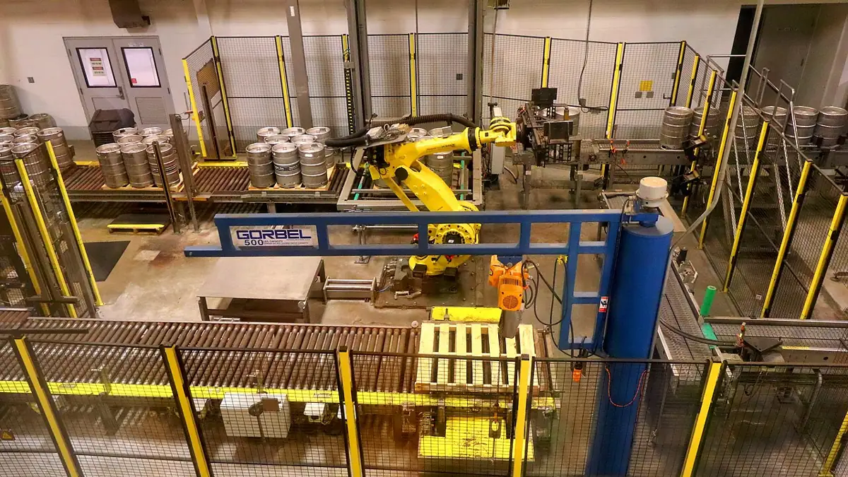
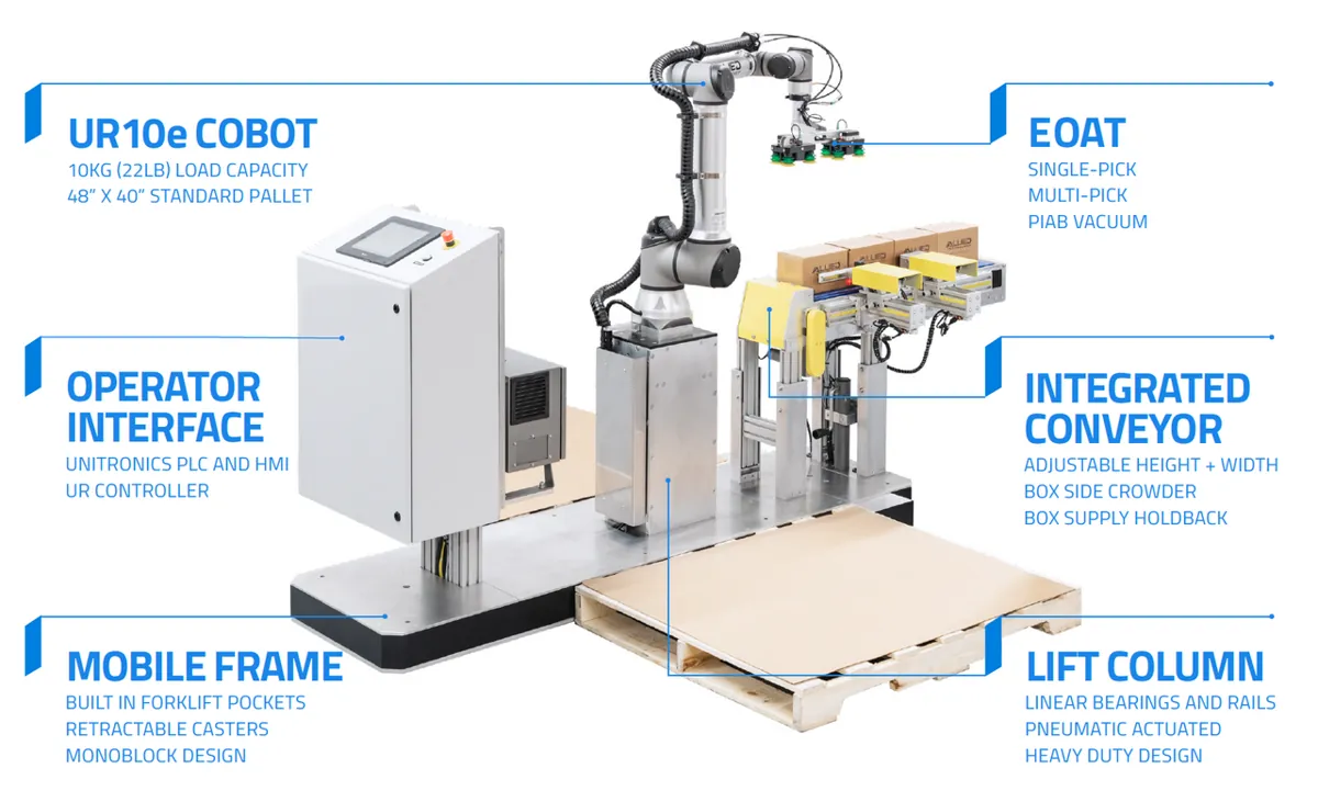
- Palletising and packing: a robot picks boxes from a conveyor and stacks them on a pallet hundreds of times an hour. Each move is planned so the box does not slide off and the cycle time stays short.
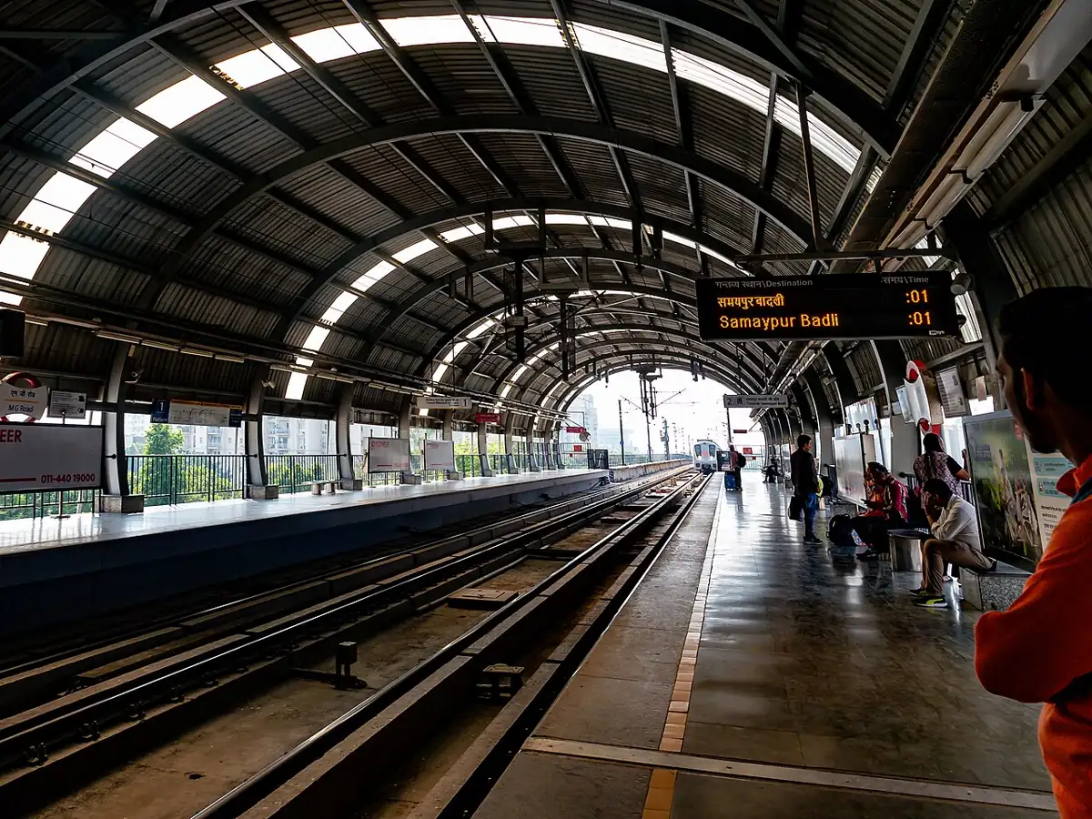
- Metro trains: a Delhi Metro train does not jump from 0 to full speed. It speeds up smoothly, cruises and brakes gently so standing passengers stay on their feet — the same idea as a trajectory with limited acceleration.
- Lifts (elevators): a good lift starts and stops so gently you barely feel it. That comfort is a designed motion profile.
- Camera sliders and gimbals: film makers use slow-in, slow-out motion so shots look smooth.
Bench build
Bench build: see and hear the difference
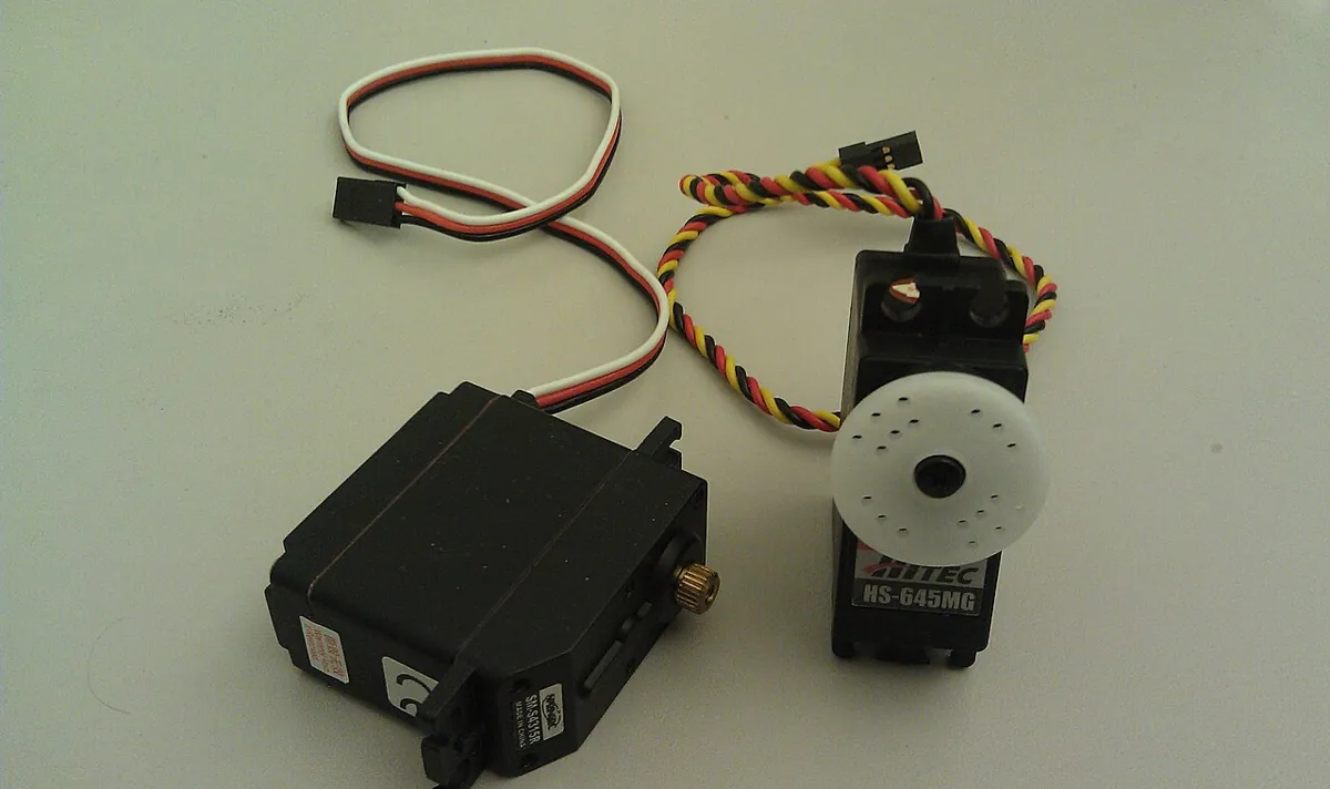
Fix a servo to a heavy block, push a 10–12 cm ice-cream-stick ‘arm’ onto its horn and tape a small coin at the tip. smooth_vs_jump.ino moves the arm between 30° and 120°. Button D2 jumps; button D3 runs the 1.5 s cubic. Watch the coin and listen to the servo.
| From | To | Note |
|---|---|---|
| Servo signal (orange/yellow) | Arduino D9 | Signal only |
| Servo + (red) | Separate 5–6 V supply + | e.g. 4×AA pack or a 5 V 2 A adapter — not the Arduino 5 V pin |
| Servo − (brown/black) | Supply − | — |
| Supply − | Arduino GND | Common ground — without it the signal has no reference |
| Push button 1 | D2 ↔ GND | Uses INPUT_PULLUP, no resistor needed |
| Push button 2 | D3 ↔ GND | Uses INPUT_PULLUP |
Mount firmly
Screw or hot-glue the servo to a heavy base. A loose servo will hop across the table on the jump test.
Upload and open Serial Monitor
Set 115200 baud. The servo goes to 30° and waits.
Press D2 (jump)
The arm snaps to 120°. Does the coin stay on? Is there a buzz or a bounce at the end?
Press D3 (smooth)
The arm glides back to 30° over 1.5 s. The Serial Monitor prints time and angle every 20 ms — copy a few lines and compare them with the cubic column of the Python output.
Change T_MOVE
Try 0.5 s and 3.0 s. Note when the coin falls off and when the motion starts to feel slow.
// smooth_vs_jump.ino — Stage 9, Lesson 1
// One servo, two ways to go from 30° to 120°:
//   press button on D2 -> JUMP   (servo.write(goal) once; servo goes as fast as it can)
//   press button on D3 -> SMOOTH (cubic trajectory over T_MOVE seconds, updated every 20 ms)
// Wiring: servo signal -> D9. Servo red/brown(black) -> SEPARATE 5–6 V supply.
//         Supply GND -> Arduino GND (common ground). Buttons D2/D3 -> GND (INPUT_PULLUP).
// Never power the servo from an Arduino pin or the 5 V pin.

#include <Servo.h>

const int SERVO_PIN = 9;
const int BTN_JUMP = 2;
const int BTN_SMOOTH = 3;
const float A_DEG = 30.0;      // pose A
const float B_DEG = 120.0;     // pose B
const float T_MOVE = 1.5;      // seconds for the smooth move
const unsigned long DT_MS = 20; // 50 Hz command rate

Servo joint;
float current = A_DEG;          // last commanded angle

float cubicAngle(float q0, float q1, float t, float T) {
  if (t <= 0) return q0;
  if (t >= T) return q1;
  float s = 3.0 * t * t / (T * T) - 2.0 * t * t * t / (T * T * T);
  return q0 + s * (q1 - q0);
}

void jumpTo(float goal) {
  Serial.print(F("JUMP to ")); Serial.println(goal);
  joint.write((int)(goal + 0.5));
  current = goal;
}

void smoothTo(float goal) {
  float start = current;
  Serial.print(F("SMOOTH ")); Serial.print(start); Serial.print(F(" -> ")); Serial.println(goal);
  unsigned long t0 = millis();
  unsigned long next = t0;
  while (true) {
    unsigned long now = millis();
    if (now < next) continue;
    next += DT_MS;
    float t = (now - t0) / 1000.0;
    float q = cubicAngle(start, goal, t, T_MOVE);
    joint.writeMicroseconds(map((long)(q * 10), 0, 1800, 544, 2400)); // finer than whole degrees
    Serial.print(t, 2); Serial.print('\t'); Serial.println(q, 1);
    if (t >= T_MOVE) break;
  }
  current = goal;
}

void setup() {
  Serial.begin(115200);
  pinMode(BTN_JUMP, INPUT_PULLUP);
  pinMode(BTN_SMOOTH, INPUT_PULLUP);
  joint.attach(SERVO_PIN);   // default 544–2400 µs range of the Servo library
  joint.write((int)A_DEG);
  delay(1000);
  Serial.println(F("D2 = jump, D3 = smooth. Each press toggles between A and B."));
}

void loop() {
  float goal = (current < (A_DEG + B_DEG) / 2) ? B_DEG : A_DEG;
  if (digitalRead(BTN_JUMP) == LOW) { jumpTo(goal); delay(800); }
  if (digitalRead(BTN_SMOOTH) == LOW) { smoothTo(goal); delay(300); }
}
Debugging
Debugging your first trajectory
| Symptom | Likely cause | Fix |
|---|---|---|
| Smooth move looks exactly like the jump | Code writes the goal, not the computed q | Make sure joint.writeMicroseconds() gets q inside the loop |
| Move takes far longer than T_MOVE | Serial.print at low baud slows the loop | Use 115200 baud or print every 5th step |
| Arm jerks at the very start | Trajectory started from a different angle than the servo was at | Start from the last commanded angle (current), as the sketch does |
| Arduino resets when the servo moves | Servo powered from the Arduino | Separate supply + common ground |
| Python peak acceleration a bit below 6·d/T² | Finite differences at 20 ms | Expected; smaller DT_CTRL gets closer to 240°/s² |
Think
Think about it
Think
Meera says, “I’ll just make T very large, like 20 seconds, then every move is gentle.” Is that a good idea for a factory robot? What are we really trading off when we choose T?
Experiment
Try it in the lab
About 30 minutes with the Python file and the browser explorer (and the optional servo bench).
Experiment
Pose versus trajectory
You will need
- `why_trajectories.py` and Python 3
- Trajectory concept explorer (in your browser)
- Notebook and pencil
- Optional: Arduino UNO, one hobby servo, separate 5–6 V supply, 2 push buttons, ice-cream stick, a coin
Steps
- Run `why_trajectories.py`. Plot (on paper or in a spreadsheet) time against the cubic angle from Part 1. Draw the jump as a second line.
- Mark on your plot where the cubic moves fastest. Check it is at t = T/2 = 0.75 s.
- Change GOAL to 60°. Predict the new peak speed with 1.5·d/T before running. Were you right?
- Change T to 0.8 s and look at Part 4. Which limit is broken first — speed or acceleration?
- In the concept explorer, scrub along the path, then toggle “hold pose” and describe the difference in one sentence.
- Optional: on the bench, find the smallest T_MOVE at which the coin still stays on the stick.
Interactive · Trajectory concept explorer
A pose is a snapshot. A trajectory is a time-parameterized path — where to be and when. Scrub progress; toggle "hold pose" to feel the difference.
The jump asks for impossible speed and acceleration; the cubic asks for modest values that you can predict before moving. Halving T doubles the peak speed but makes the peak acceleration four times larger, because acceleration depends on 1/T².
Knowledge check
Check your understanding
Knowledge check
1. A trajectory is best described as…
2. Which one has **no** notion of time?
3. Your command jumps 90° in one 20 ms step. What speed are you asking for?
4. For a rest-to-rest cubic, where is the speed highest?
5. You halve the move time T. The peak acceleration of the cubic becomes…
6. Where does trajectory planning fit between Stage 8 IK and the Stage 7 PID loop?
7. Why must the servo in the bench build use a separate supply?
Mini assignment
Hands-on assignment
Mini assignment
Jump vs trajectory report
Prove, with numbers and a plot, why a robot needs a trajectory — using one joint of your own arm.
Deliverables
- Pick one real joint of your Stage 6 arm (or the bench servo) and choose a start angle, goal angle and T.
- Run `why_trajectories.py` with your numbers and attach the output.
- A hand-drawn or spreadsheet plot of angle vs time for both the jump and the cubic.
- Using the formulas, find the smallest T that keeps peak speed ≤ 120°/s and peak acceleration ≤ 300°/s² (or your own servo’s limits, if you know them). Show your working.
- Three sentences: what a pose, a path and a trajectory are, in your own words, with an everyday example of each.
- Optional: a short phone video of the bench build doing a jump and then a smooth move.
Do this, step by step
- Run
python3 why_trajectories.pyand copy Part 2. Circle the peak speed and peak acceleration of the jump and of the cubic. - Change
START, GOALto your own joint’s angles. Before running, predict the cubic’s peak speed with 1.5·d/T and write it down. Run and compare. - Change
Tto 0.8 and read Part 4. Write which limit breaks first — speed or acceleration — and why (hint: 1/T²). - Find the smallest
Tthat passes Part 4 for your move by trying values 0.1 s apart. Check it against the formula answer. - Optional bench: upload
smooth_vs_jump.ino, press D2 then D3 with the coin on the stick, and note the shortestT_MOVEat which the coin stays on.
Stuck? Hints, one at a time
- d is the change in angle, GOAL − START. For 30° → 120°, d = 90°.
- Peak speed = 1.5·d/T and peak acceleration = 6·d/T². Solve each for T and keep the larger T.
- If the coin still falls at a long T_MOVE, check that the servo base is fixed firmly — a hopping base adds its own shake.
Challenges (pick by level)
- 🟢 Easy: Compute by hand the cubic angle at t = T/2 for 30° → 120°. (Hint: s = 0.5.)
- 🟢 Easy: List four machines in your home or city that start and stop gently, and say what would go wrong if they jumped.
- 🟡 Medium: Add a third plan to the Python file: a straight-line (constant-speed) move. Compare its peak acceleration with the cubic.
- 🟠 Hard-ish: Change the sketch so a single button press does 30° → 120° → 30° as one smooth back-and-forth, without a stop in the middle bigger than 0.2 s.
- 🔴 Hard: Solve the two formulas for T to get the smallest feasible T directly from the speed limit and from the acceleration limit, and take the larger one. Code it as
min_time(d, vlim, alim). - ⚫ Research: Read Section 9.1–9.2 of *Modern Robotics* and write down the difference between a “path” and a “time scaling” in the book’s words.
Next step
Before we plan motions for many joints at once, we need a clear picture of “all the possible configurations” of a robot. In Lesson 2 — Configuration Space & Robot Motion you will draw a 2-joint arm’s whole world as a single square map.
Look back: Stage 8: Capstone: Design & Solve the Kinematics. Next: Lesson 2: Configuration Space & Robot Motion. Related: Stage 7 — Control Systems & PID and Stage 10 — ROS 2.
Sources
- Modern Robotics (Lynch & Park) — book home page and free PDF — Chapter 9: trajectory = path + time scaling; rest-to-rest cubic, peak speed 1.5·d/T and peak acceleration 6·d/T².
- Modern Robotics video — 9.1 and 9.2 Point-to-Point Trajectories — companion lecture for the same sections.
- Wikipedia — Motion planning — motion (path) planning as finding a sequence of valid configurations from start to goal.
- Arduino — Servo library —
attach(),write()andwriteMicroseconds()used in the bench sketch. - Photos and drawing: Wikimedia Commons (credits under each image).
Self-attested for now — keep artifacts in your lab notebook.
Complete
Today's goal
0 of 1 done today
Mark this lesson complete when you have worked the experiment, knowledge check, and assignment (even roughly).