
Trajectory Planning & Motion Generation · Lesson 05
Waypoints & Motion Segments
Est. 50–70 min
Why
Why this lesson matters
Real robot jobs are almost never a single start → goal move. They are a list of waypoints (also called via points) — poses the robot must pass through — joined by segments, each with its own duration. How you treat each waypoint matters a lot: stop dead, or flow through? Equal timing for every segment, or more time for longer ones? These choices decide the cycle time, the smoothness and the wear on the motors.
By the end of this lesson you will be able to: write a task as a waypoint table in task space and convert it to joint space with IK; time each segment; join segments with cubic via-point polynomials that keep position and velocity continuous; compare stopping at every waypoint with flowing through them; see why plain straight-line segments give velocity jumps at every corner; and play a waypoint job on a 2-servo arm with a HOLD button.
Concept
A job is a list of stops
Waypoints, segments and via velocities
| Word | Meaning | Pick-and-place example |
|---|---|---|
| Waypoint (via point) | A pose the robot must pass through | “above pick” at tip (13, 4) cm |
| Segment | The motion between two neighbouring waypoints | “above pick” → “pick” |
| Segment time ΔT | How long that segment takes | 0.6 s for the short drop |
| Via velocity | The joint speed the robot should have as it passes the waypoint | 0 (stop) or, say, −31°/s (flow through) |
A good waypoint list usually has approach and retreat points: you never go straight to “pick”; you go to “above pick” first, then a short, slow, straight move down, then back up. This keeps the gripper from sweeping sideways into the object, and gives a natural place to check the gripper is open or closed.
Joining segments: the cubic via-point polynomial
*Modern Robotics* (Section 9.3) gives a neat recipe. For each segment j, with start position q_j, end position q_{j+1}, start velocity v_j, end velocity v_{j+1} and duration ΔT, use a cubic with these coefficients:
q(t) = a0 + a1·t + a2·t² + a3·t³,   0 ≤ t ≤ ΔT
a0 = q_j
a1 = v_j
a2 = (3·q_{j+1} − 3·q_j − 2·v_j·ΔT − v_{j+1}·ΔT) / ΔT²
a3 = (2·q_j + (v_j + v_{j+1})·ΔT − 2·q_{j+1}) / ΔT³- Because each segment starts with the velocity the previous one ended with, position and velocity are continuous at every waypoint — no jumps.
- Acceleration is not continuous at the waypoints with cubics. If you need that too, the same idea works with fifth-order (quintic) segments — Lesson 8.
- If you set every via velocity to 0, each segment becomes the rest-to-rest cubic from Lesson 1: the robot stops at every waypoint.
- The book also notes that sensible choices of via times and velocities make the motion much smoother — a simple rule is “average of the slopes on either side, but 0 where the joint reverses direction”.
Visual
Visualise it: segments between waypoints
Scrub along a path through several waypoints. Each stretch between two waypoints is one segment with its own timing.
Interactive · Trajectory concept explorer


A pose is a snapshot. A trajectory is a time-parameterized path — where to be and when. Scrub progress; toggle "hold pose" to feel the difference.
Code lab
Code lab: a pick-and-place job as waypoints
waypoints.py writes a 7-waypoint pick-and-place job for the Stage 8 arm in task space, converts every waypoint to joint angles with IK, and then compares three ways of joining them: stop everywhere (Plan A), flow through where possible (Plan B), and plain constant-speed lines (Plan C). Run python3 waypoints.py.
"""waypoints.py — Stage 9, Lesson 5
A pick-and-place job for the 2-link arm (L1 = 10 cm, L2 = 8 cm) written as WAYPOINTS,
joined by timed SEGMENTS. Each segment is a cubic (Modern Robotics 9.3, eq. 9.26-9.29):
    a0 = q_j, a1 = v_j,
    a2 = (3 q_j+1 - 3 q_j - 2 v_j dT - v_j+1 dT) / dT^2,
    a3 = (2 q_j + (v_j + v_j+1) dT - 2 q_j+1) / dT^3
Plan A: stop at every waypoint (all via velocities = 0).
Plan B: keep moving through the middle waypoints (via velocities from a simple rule).
Plan C: straight-line segments at constant speed (velocity jumps at every corner).
"""
import math

L1, L2 = 10.0, 8.0


def ik(x, y):
    c2 = (x * x + y * y - L1 * L1 - L2 * L2) / (2 * L1 * L2)
    t2 = math.acos(max(-1.0, min(1.0, c2)))
    t1 = math.atan2(y, x) - math.atan2(L2 * math.sin(t2), L1 + L2 * math.cos(t2))
    return math.degrees(t1), math.degrees(t2)


# name, tip (x, y) in cm, time to reach it from the previous waypoint (s)
TASK = [
    ("home",        (6.0, 12.0), 0.0),
    ("above pick",  (13.0, 4.0), 1.2),
    ("pick",        (13.0, 1.0), 0.6),
    ("above pick",  (13.0, 4.0), 0.6),
    ("above place", (-6.0, 13.0), 1.6),
    ("place",       (-6.0, 10.0), 0.6),
    ("home",        (6.0, 12.0), 1.2),
]
Q = [ik(*p) for _, p, _ in TASK]
DT = [d for _, _, d in TASK[1:]]

print("Part 1 - the waypoint table (task space -> joint space with IK)")
print(" #  name          tip (x, y) cm     theta1   theta2   seg time")
for i, ((name, p, d), q) in enumerate(zip(TASK, Q)):
    print(f"{i:2d}  {name:12s} ({p[0]:5.1f}, {p[1]:5.1f})   {q[0]:7.1f}  {q[1]:7.1f}   {d:4.1f} s")
print(f"segments: {len(DT)}, total time {sum(DT):.1f} s")


def via_velocities(qs, dts, stop_everywhere):
    """Rule: 0 at the ends; in the middle, average of the two neighbouring slopes,
    but 0 if the joint changes direction there (so it does not overshoot)."""
    v = [0.0] * len(qs)
    if stop_everywhere:
        return v
    for i in range(1, len(qs) - 1):
        s1 = (qs[i] - qs[i - 1]) / dts[i - 1]
        s2 = (qs[i + 1] - qs[i]) / dts[i]
        v[i] = 0.0 if s1 * s2 <= 0 else 0.5 * (s1 + s2)
    return v


def cubic_seg(q0, q1, v0, v1, d, t):
    a2 = (3 * q1 - 3 * q0 - 2 * v0 * d - v1 * d) / d**2
    a3 = (2 * q0 + (v0 + v1) * d - 2 * q1) / d**3
    return (q0 + v0 * t + a2 * t * t + a3 * t**3,
            v0 + 2 * a2 * t + 3 * a3 * t * t,
            2 * a2 + 6 * a3 * t)


def analyse(name, stop_everywhere):
    print(f"\n{name}")
    for j in range(2):
        qs = [q[j] for q in Q]
        v = via_velocities(qs, DT, stop_everywhere)
        peak_v = peak_a = 0.0
        for k in range(len(DT)):
            for n in range(101):
                t = DT[k] * n / 100
                _, vel, acc = cubic_seg(qs[k], qs[k + 1], v[k], v[k + 1], DT[k], t)
                peak_v, peak_a = max(peak_v, abs(vel)), max(peak_a, abs(acc))
        stops = sum(1 for x in v[1:-1] if x == 0)
        print(f"  joint {j+1}: via velocities {[round(x) for x in v]} deg/s")
        print(f"           stops at {stops} of {len(v)-2} middle waypoints, peak |v| {peak_v:6.1f} deg/s, peak |a| {peak_a:7.1f} deg/s^2")


analyse("Part 2 - Plan A: stop at every waypoint", True)
analyse("Part 3 - Plan B: flow through middle waypoints where the joint keeps its direction", False)

print("\nPart 4 - Plan C: constant-speed straight segments (no smoothing)")
for j in range(2):
    sp = [(Q[k + 1][j] - Q[k][j]) / DT[k] for k in range(len(DT))]
    jumps = [abs(sp[0])] + [abs(sp[k] - sp[k - 1]) for k in range(1, len(sp))] + [abs(sp[-1])]
    print(f"  joint {j+1}: segment speeds {[round(s) for s in sp]} deg/s")
    print(f"           biggest instant speed change at a corner: {max(jumps):.0f} deg/s (infinite acceleration)")

print("\nPart 5 - check: does every segment start where the last one ended?")
ok = all(abs(cubic_seg(Q[k][j], Q[k+1][j], 0, 0, DT[k], DT[k])[0] - Q[k+1][j]) < 1e-9
         for k in range(len(DT)) for j in range(2))
print("position continuous at all waypoints:", ok)
Output (run with python3 waypoints.py)
Part 1 - the waypoint table (task space -> joint space with IK)
 #  name          tip (x, y) cm     theta1   theta2   seg time
 0  home         (  6.0,  12.0)      27.0     84.3    0.0 s
 1  above pick   ( 13.0,   4.0)     -18.6     82.5    1.2 s
 2  pick         ( 13.0,   1.0)     -33.4     87.9    0.6 s
 3  above pick   ( 13.0,   4.0)     -18.6     82.5    0.6 s
 4  above place  ( -6.0,  13.0)      82.1     75.2    1.6 s
 5  place        ( -6.0,  10.0)      78.5    100.1    0.6 s
 6  home         (  6.0,  12.0)      27.0     84.3    1.2 s
segments: 6, total time 5.8 s

Part 2 - Plan A: stop at every waypoint
  joint 1: via velocities [0, 0, 0, 0, 0, 0, 0] deg/s
           stops at 5 of 5 middle waypoints, peak |v|   94.4 deg/s, peak |a|   247.6 deg/s^2
  joint 2: via velocities [0, 0, 0, 0, 0, 0, 0] deg/s
           stops at 5 of 5 middle waypoints, peak |v|   62.3 deg/s, peak |a|   415.4 deg/s^2

Part 3 - Plan B: flow through middle waypoints where the joint keeps its direction
  joint 1: via velocities [0, -31, 0, 44, 0, -24, 0] deg/s
           stops at 2 of 5 middle waypoints, peak |v|   85.4 deg/s, peak |a|   181.1 deg/s^2
  joint 2: via velocities [0, 0, 0, -7, 0, 0, 0] deg/s
           stops at 4 of 5 middle waypoints, peak |v|   62.3 deg/s, peak |a|   415.4 deg/s^2

Part 4 - Plan C: constant-speed straight segments (no smoothing)
  joint 1: segment speeds [-38, -25, 25, 63, -6, -43] deg/s
           biggest instant speed change at a corner: 69 deg/s (infinite acceleration)
  joint 2: segment speeds [-2, 9, -9, -5, 42, -13] deg/s
           biggest instant speed change at a corner: 55 deg/s (infinite acceleration)

Part 5 - check: does every segment start where the last one ended?
position continuous at all waypoints: TrueTry it: each cubic segment is one stretch between two waypoints. Change start, goal and T and watch velocity stay continuous and zero at the ends.
Interactive · Cubic trajectory lab


Rest-to-rest cubic: q(0)=q₀, q(T)=q_f, q̇(0)=q̇(T)=0 → unique coefficients. Compare to linear lerp: cubic has continuous velocity (zero at ends) — kinder to motors and PID.
Position · q(t)
Velocity · q̇(t)
Acceleration · q̈(t)
q
34.6°
q̇
40.3°/s
q̈
13.4°/s²
Peak |q̇| scales ~1/T; peak |q̈| ~1/T². Shorten T → hotter motors / harder PID. Quintics (Part 2) also match acceleration at boundaries.
Real world
Waypoints in the real world
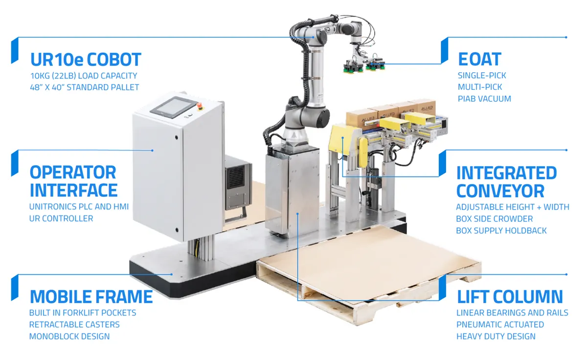
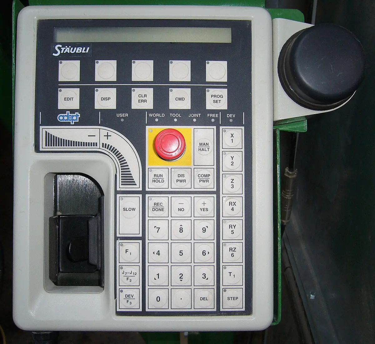
- Industrial robots: a program is a list of stored positions with a move type and speed for each. In ABB’s RAPID, for example, the zone data of each move says whether that point is a stop point or a fly-by point that the robot may round off.
- Drones: autopilots such as ArduPilot fly missions that are planned as a list of waypoints and events, uploaded before take-off.
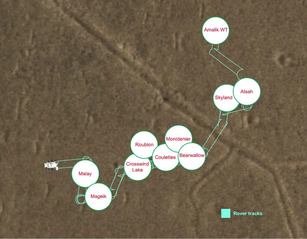
- Mars rovers: NASA’s Perseverance drove between planned stops to drop each of its sample tubes at the “Three Forks” depot — a waypoint list on another planet.
- CNC and 3D printing: G-code is a long list of points; the firmware’s planner joins them into smooth segments and decides how much to slow at each corner.
Bench build
Bench build: a waypoint player with a HOLD button
Use the 2-servo arm from Lesson 4. waypoint_player.ino contains the joint table printed by waypoints.py and plays the whole job in a loop. Set FLOW = false for Plan A or true for Plan B. Holding the D2 button freezes the arm in place mid-segment — your first “feed hold”.
| From | To | Note |
|---|---|---|
| Shoulder servo signal | D9 | Shoulder servo angle = θ₁ + 60° |
| Elbow servo signal | D10 | Elbow servo angle = θ₂ |
| Both servos + and − | Separate 5–6 V supply, 2 A or more | Never the Arduino 5 V pin |
| Supply − | Arduino GND | Common ground |
| HOLD button | D2 ↔ GND | INPUT_PULLUP |
Mark the job on paper
Draw the 5 tip positions (home, above pick, pick, above place, place) on chart paper under the arm, measured from the shoulder axis.
Run Plan A
Upload with FLOW = false. Watch the arm stop at every mark. Time one full cycle with a phone stopwatch.
Run Plan B
Upload with FLOW = true. The cycle time is the same, but the shoulder should glide through the marks where it does not reverse. Listen: is it quieter?
Test HOLD
Press and hold D2 mid-swing. The arm freezes; release and it continues exactly where it left off, because the segment clock is paused too.
// waypoint_player.ino — Stage 9, Lesson 5
// Plays a pick-and-place job on a 2-servo arm as a list of joint WAYPOINTS joined by
// cubic SEGMENTS (Modern Robotics eq. 9.26–9.29). The table is the output of waypoints.py.
//   FLOW = false : stop at every waypoint (Plan A)
//   FLOW = true  : keep moving through middle waypoints where a joint keeps its direction (Plan B)
// Button on D2 (to GND) = HOLD: while pressed, the arm freezes where it is.
//
// Wiring: shoulder servo signal -> D9, elbow servo signal -> D10.
//         Servo power from a SEPARATE 5–6 V supply (2 A+); supply GND -> Arduino GND.
//         Never power servos from an Arduino pin or the 5 V pin.
// Mounting: shoulder servo angle = theta1 + 60 (so theta1 = -60..120 fits 0..180); elbow servo = theta2.

#include <Servo.h>

const bool FLOW = false;
const int N = 7;
const char* NAMES[N] = {"home", "above pick", "pick", "above pick", "above place", "place", "home"};
const float Q[N][2] = {
  {27.0, 84.3}, {-18.6, 82.5}, {-33.4, 87.9}, {-18.6, 82.5}, {82.1, 75.2}, {78.5, 100.1}, {27.0, 84.3}
};
const float DTSEG[N - 1] = {1.2, 0.6, 0.6, 1.6, 0.6, 1.2};   // seconds per segment
const float SH_OFFSET = 60.0;
const unsigned long STEP_MS = 20;

Servo sh, el;
float V[N][2];   // via velocities, deg/s

void writeJoint(Servo &s, float servoDeg) {
  servoDeg = constrain(servoDeg, 0, 180);
  s.writeMicroseconds(544 + (long)(servoDeg * (2400 - 544) / 180.0));
}

void command(float t1, float t2) {
  writeJoint(sh, t1 + SH_OFFSET);
  writeJoint(el, t2);
}

void computeVias() {
  for (int j = 0; j < 2; j++) {
    V[0][j] = V[N - 1][j] = 0;
    for (int i = 1; i < N - 1; i++) {
      float s1 = (Q[i][j] - Q[i - 1][j]) / DTSEG[i - 1];
      float s2 = (Q[i + 1][j] - Q[i][j]) / DTSEG[i];
      V[i][j] = (!FLOW || s1 * s2 <= 0) ? 0 : 0.5 * (s1 + s2);
    }
  }
}

float cubicPos(float q0, float q1, float v0, float v1, float d, float t) {
  float a2 = (3 * q1 - 3 * q0 - 2 * v0 * d - v1 * d) / (d * d);
  float a3 = (2 * q0 + (v0 + v1) * d - 2 * q1) / (d * d * d);
  return q0 + v0 * t + a2 * t * t + a3 * t * t * t;
}

void setup() {
  Serial.begin(115200);
  pinMode(2, INPUT_PULLUP);
  sh.attach(9);
  el.attach(10);
  computeVias();
  command(Q[0][0], Q[0][1]);
  delay(2000);
}

void loop() {
  for (int k = 0; k < N - 1; k++) {
    Serial.print(F("segment ")); Serial.print(k + 1); Serial.print(F(": "));
    Serial.print(NAMES[k]); Serial.print(F(" -> ")); Serial.println(NAMES[k + 1]);
    float t = 0;
    while (t <= DTSEG[k]) {
      if (digitalRead(2) == LOW) { delay(STEP_MS); continue; }   // HOLD: time does not advance
      float t1 = cubicPos(Q[k][0], Q[k + 1][0], V[k][0], V[k + 1][0], DTSEG[k], t);
      float t2 = cubicPos(Q[k][1], Q[k + 1][1], V[k][1], V[k + 1][1], DTSEG[k], t);
      command(t1, t2);
      delay(STEP_MS);
      t += STEP_MS / 1000.0;
    }
    command(Q[k + 1][0], Q[k + 1][1]);   // land exactly on the waypoint
  }
  Serial.println(F("job done - waiting 3 s"));
  delay(3000);
}
Debugging
Debugging waypoint jobs
| Symptom | Likely cause | Fix |
|---|---|---|
| Arm jumps at the start of a segment | Segment does not start at the previous segment’s end | Use the same waypoint value for “end of j” and “start of j+1” |
| Overshoot past a waypoint, then come back | Non-zero via velocity where the joint reverses | Use 0 via velocity where the slope changes sign |
| One segment is violent, others calm | Same ΔT for a long and a short segment | Scale ΔT with the joint change; check peaks |
| Gripper sweeps the object sideways | No approach / retreat waypoints | Add “above pick” and “above place” |
| Arm flips elbow between waypoints | IK returned different branches for neighbouring waypoints | Use one branch for the whole job |
Think
Think about it
Think
In Plan B, joint 2 still stops at 4 of the 5 middle waypoints. Ananya says, “Let’s just give it a non-zero via velocity everywhere so it never stops.” What could go wrong?
Experiment
Try it in the lab
About 35 minutes with waypoints.py and the browser labs; the 2-servo player is optional.
Experiment
Stops versus flow
You will need
- `waypoints.py` and Python 3
- Graph paper or a spreadsheet
- Cubic trajectory lab and trajectory explorer (in your browser)
- Optional: 2-servo arm from Lesson 4, separate 5–6 V 2 A supply, one push button
Steps
- Run `waypoints.py`. Draw the 7 tip positions on graph paper and number the segments.
- Change the long swing (segment 4) from 1.6 s to 1.0 s. Which peak values change in Plan A, and by how much?
- Change it back and instead make every segment 1.0 s. Is the job faster? Which segment now has the highest acceleration?
- Add a new waypoint “lift high” at (8, 14) between “above pick” and “above place”. How do the via velocities change?
- In Part 3, print joint 1’s position every 0.1 s for Plan A and Plan B and plot both. Where do they differ most?
- Optional: run both plans on the servo arm and compare sound and smoothness. Test the HOLD button.
Interactive · Cubic trajectory lab
Rest-to-rest cubic: q(0)=q₀, q(T)=q_f, q̇(0)=q̇(T)=0 → unique coefficients. Compare to linear lerp: cubic has continuous velocity (zero at ends) — kinder to motors and PID.
Position · q(t)
Velocity · q̇(t)
Acceleration · q̈(t)
q
34.6°
q̇
40.3°/s
q̈
13.4°/s²
Peak |q̇| scales ~1/T; peak |q̈| ~1/T². Shorten T → hotter motors / harder PID. Quintics (Part 2) also match acceleration at boundaries.
Cubic via-point segments keep position and velocity continuous. Flowing through waypoints where a joint keeps its direction lowers peak acceleration for the same total time. Constant-speed straight segments jump in velocity at every corner. Segment times should reflect segment lengths.
Knowledge check
Check your understanding
Knowledge check
1. A waypoint (via point) is…
2. Why add an “above pick” waypoint before “pick”?
3. With cubic via-point segments, which are continuous at every waypoint?
4. If every via velocity is set to 0, the robot…
5. In `waypoints.py`, what happened to joint 1’s peak acceleration from Plan A to Plan B?
6. Constant-speed straight segments joined at corners cause…
7. A good rule for a joint’s via velocity at a waypoint where it reverses direction is…
Mini assignment
Hands-on assignment
Mini assignment
Design your own waypoint job
Plan a small task for your arm as a waypoint table, time it, and compare stopping with flowing — then run it.
Deliverables
- Choose a task (e.g. move an eraser from one box to another). Write the waypoint table: name, tip (x, y), segment time. Include approach and retreat points.
- Put your table into `waypoints.py` and attach the output for Plan A and Plan B.
- Explain one change you made to a segment time and why (use the peak values).
- Sketch the job on graph paper with numbered waypoints and arrows for segments.
- Copy your joint table into `waypoint_player.ino` and record a short video or write what you observed.
Do this, step by step
- Run
python3 waypoints.pyand copy the Part 1 waypoint table (task space → joints). - Compare Plan A (stop at every waypoint) and Plan B (flow through) in Parts 2–3. Write the cycle time and the peak acceleration for both.
- Edit
TASKwith your own pick-and-place points, including an approach point above the pick and a retreat point. - Change one segment time and re-run. Write how the peak values changed and whether Part 5’s continuity check still passes.
- Optional bench: copy your joint table into
Qinwaypoint_player.ino, tryFLOWon and off, and write what you see at each waypoint.
Stuck? Hints, one at a time
- A waypoint is a pose the robot must pass through; a segment is the motion between two waypoints.
- Approach and retreat points keep the gripper moving straight down and up, so it does not sweep into the object.
- If Part 5 fails, the end of one segment and the start of the next do not match — check the order of rows in TASK.
Challenges (pick by level)
- 🟢 Easy: Write the waypoints of your morning route to school or college, and mark which are full stops and which are roll-throughs.
- 🟢 Easy: Count the segments in a job with 9 waypoints.
- 🟡 Medium: Make
waypoints.pychoose each segment time automatically so that no segment’s peak speed exceeds 60°/s in Plan A. - 🟠 Hard-ish: Add a check that every intermediate sample of every segment stays within joint limits (shoulder −60° to 120°, elbow 0° to 150°).
- 🔴 Hard: Implement Plan B in task space instead: interpolate x and y with via-point cubics, run IK at each sample, and compare the tool path with the joint-space version.
- ⚫ Research: Read *Modern Robotics* §9.3 on via-point trajectories and B-splines. Why might a path that stays inside the “convex hull” of the via points be safer?
Next step
You have used “straight line between two values” many times now. In Lesson 6 — Linear Interpolation you will study it properly: the lerp formula, where it shines, and exactly why its corners need help.
Look back: Lesson 4: Joint-Space vs Cartesian-Space Motion. Next: Lesson 6: Linear Interpolation. Related: Stage 6 — 6DOF Arm.
Sources
- Modern Robotics (Lynch & Park) — book home page and free PDF — §9.3 Polynomial via point trajectories: cubic segment coefficients (eq. 9.26–9.29), continuity of position and velocity but not acceleration, choosing via times/velocities, B-splines and the convex hull.
- Wikipedia — Motion planning — a motion as a sequence of valid configurations.
- ABB RAPID summary — Motion (RobotStudio course page) — pose-to-pose programming; zonedata sets a stop point or fly-by point.
- ArduPilot — Planning a Mission with Waypoints and Events — drone missions as waypoint lists.
- Arduino — Servo library —
writeMicroseconds()used by the waypoint player. - Photos and map: Wikimedia Commons (credits under each image).
Self-attested for now — keep artifacts in your lab notebook.
Complete
Today's goal
0 of 1 done today
Mark this lesson complete when you have worked the experiment, knowledge check, and assignment (even roughly).