
Control Systems & PID · Lesson 09
Step Response Metrics
Est. 60–75 min
Why
Why “it looks good” is not good enough
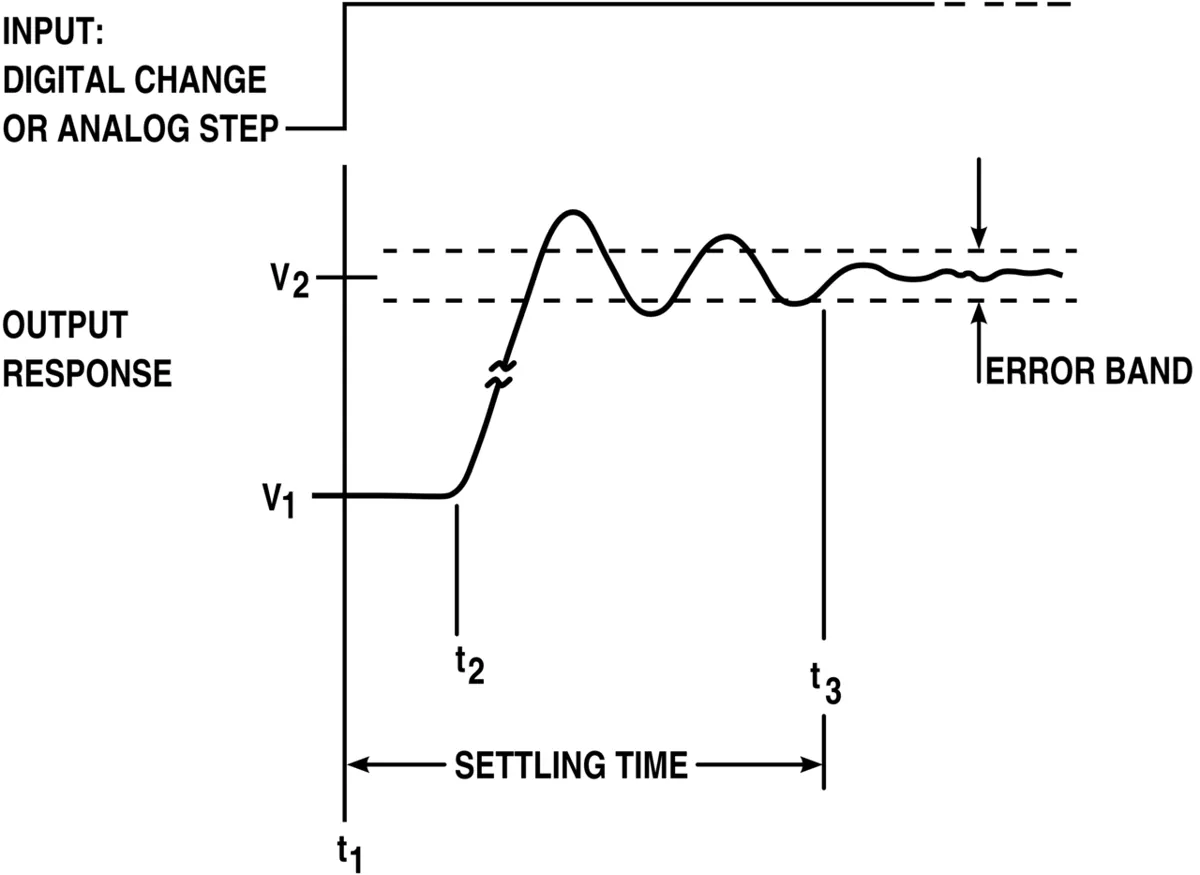
In Lessons 5–8 you saw tables with peaks, overshoot percentages and settling times. This lesson makes those numbers precise. A step response is what the system does when the setpoint jumps suddenly (for example, 0° → 90°). The Michigan *Control Tutorials* define the standard measurements: rise time (usually 10 % → 90 % of the final value), settling time (time to stay within a band such as 2 % of the final value), and percent overshoot (how far the response goes past its final value). Add the peak and steady-state error and you have a clear report card for any controller.
By the end of this lesson you will be able to: define the five metrics exactly; compute them in code from logged data; explain why overshoot is measured against the *final value*, not the setpoint; record a real step response from the LED + LDR bench at a fixed sample rate; and spot common measurement traps (noise, too-short logs, wrong band).
Concept
The five numbers that describe a step response
| Metric | What it means | How to measure it |
|---|---|---|
| Rise time | How quickly the response gets going | Time from 10 % to 90 % of the final value |
| Peak (and time to peak) | Highest value reached | max(y) and when it happened |
| Percent overshoot | How far it goes past the final value | (peak − final) ÷ (final − start) × 100 |
| Settling time | When it calms down | Last time it is outside ±2 % of the final value |
| Steady-state error | How far from the target it ends | setpoint − final value |
The table below uses the same joint as the earlier lessons and the metrics() function in this lesson’s code. Now all four controllers are compared on one fair scale.
| Controller | Rise (10–90 %) | Peak | Overshoot | Settling (2 %) | Final | SSE |
|---|---|---|---|---|---|---|
| P, Kp = 0.01 | 0.69 s | 102.65° | 20.8 % | 3.73 s | 85.00° | 5.00° |
| P, Kp = 0.04 | 0.28 s | 131.90° | 48.6 % | 3.78 s | 88.75° | 1.25° |
| PD, Kd = 0.008 | 0.46 s | 93.89° | 5.8 % | 1.34 s | 88.75° | 1.25° |
| PID, Ki = 0.002, Kd = 0.008 | 0.46 s | 95.35° | 5.9 % | 1.35 s | 90.07° | −0.07° |
Read it like a report card. Kp = 0.04 has the fastest rise (0.28 s) but terrible overshoot. PD trades a little rise time for much less overshoot and faster settling. PID keeps PD’s good numbers *and* removes the steady-state error. One table, no arguing.
Final value vs setpoint
The *Control Tutorials* define percent overshoot against the final steady-state value. If the response never reaches the setpoint (PD stops at 88.75°), measuring against the setpoint gives a different number: 4.3 % instead of 5.8 % for the same curve. Neither is “wrong”, but you must say which one you used — otherwise two teams can report different numbers for the same robot.
Visual
Visualise it: read the metrics off a curve
Change the controller and read the **rise time, overshoot and settling time**. Try to improve one metric without making another one worse.
Interactive · Control response lab
Goal: |SSE| ≤ 2°, overshoot ≤ 15% · Hint: Moderate Kp, light Kd, tiny Ki
|SSE|
0.24°
Overshoot
32.7%
Result
RETRY
Code lab
Code lab: a metrics() function you can reuse
step_metrics.py simulates four controllers on the same joint and measures each response with one metrics() function. You can reuse this function on any logged data — including the CSV from the bench build. Run it with python3 step_metrics.py.
# step_metrics.py - measure a step response properly: rise time, peak, overshoot,
# settling time and steady-state error. Same joint as Lessons 5-8 (angles in degrees).

J, B, LOAD, TAU_MAX = 0.002, 0.004, 0.05, 4.0
SETPOINT, DT, T_END = 90.0, 0.001, 10.0


def simulate(kp, ki, kd):
    angle = speed = integral = t = 0.0
    prev = angle
    ts, ys = [], []
    while t < T_END:
        e = SETPOINT - angle
        integral += e * DT
        d_meas = (angle - prev) / DT
        prev = angle
        torque = max(-TAU_MAX, min(TAU_MAX, kp * e + ki * integral - kd * d_meas))
        speed += (torque - B * speed - LOAD) / J * DT
        angle += speed * DT
        t += DT
        ts.append(t)
        ys.append(angle)
    return ts, ys


def metrics(ts, ys, setpoint, start=0.0, band_pct=2.0):
    """Classic step-response numbers, measured against the FINAL value."""
    final = sum(ys[-200:]) / 200            # average the last 0.2 s as the final value
    span = final - start
    t10 = next(t for t, y in zip(ts, ys) if y >= start + 0.1 * span)
    t90 = next(t for t, y in zip(ts, ys) if y >= start + 0.9 * span)
    peak = max(ys)
    t_peak = ts[ys.index(peak)]
    overshoot = max(0.0, (peak - final) / span * 100)
    band = abs(span) * band_pct / 100
    t_settle = 0.0
    for t, y in zip(ts, ys):
        if abs(y - final) > band:
            t_settle = t
    return dict(rise=t90 - t10, peak=peak, t_peak=t_peak, overshoot=overshoot,
                settle=t_settle, final=final, sse=setpoint - final)


print("Step 0 -> 90 deg on the same joint. Rise = 10-90 %, settling = within 2 % of final value\n")
print(f"{'controller':>22} {'rise':>7} {'peak':>9} {'t_peak':>7} {'overshoot':>9} {'settle':>7} {'final':>8} {'SSE':>7}")
for name, gains in (("P  Kp=0.01", (0.01, 0, 0)),
                    ("P  Kp=0.04", (0.04, 0, 0)),
                    ("PD Kp=0.04 Kd=0.008", (0.04, 0, 0.008)),
                    ("PID Ki=0.002 Kd=0.008", (0.04, 0.002, 0.008))):
    m = metrics(*simulate(*gains), SETPOINT)
    print(f"{name:>22} {m['rise']:>6.2f}s {m['peak']:>8.2f}° {m['t_peak']:>6.2f}s "
          f"{m['overshoot']:>8.1f}% {m['settle']:>6.2f}s {m['final']:>7.2f}° {m['sse']:>6.2f}°")

print("\nCareful: the same response, judged against the SETPOINT instead of the final value:")
ts, ys = simulate(0.04, 0, 0.008)
peak = max(ys)
print(f"  PD overshoot vs final value: {(peak - ys[-1]) / ys[-1] * 100:.1f} %"
      f"   vs setpoint: {(peak - SETPOINT) / SETPOINT * 100:.1f} %")
print("Always write down which definition you used.")
Output (run with python3 step_metrics.py)
Step 0 -> 90 deg on the same joint. Rise = 10-90 %, settling = within 2 % of final value

            controller    rise      peak  t_peak overshoot  settle    final     SSE
            P  Kp=0.01   0.69s   102.65°   1.57s     20.8%   3.73s   85.00°   5.00°
            P  Kp=0.04   0.28s   131.90°   0.72s     48.6%   3.78s   88.75°   1.25°
   PD Kp=0.04 Kd=0.008   0.46s    93.89°   0.95s      5.8%   1.34s   88.75°   1.25°
 PID Ki=0.002 Kd=0.008   0.46s    95.35°   0.95s      5.9%   1.35s   90.07°  -0.07°

Careful: the same response, judged against the SETPOINT instead of the final value:
  PD overshoot vs final value: 5.8 %   vs setpoint: 4.3 %
Always write down which definition you used.Try it: change the gains and read rise time, overshoot and settling time off the response. Compare two settings with numbers, not looks.
Interactive · Control response lab
Goal: |SSE| ≤ 2°, overshoot ≤ 15% · Hint: Moderate Kp, light Kd, tiny Ki
|SSE|
0.24°
Overshoot
32.7%
Result
RETRY
Simulator
Try it in the simulator
Simulator · Control
PID tuning on a DC-motor position plant
Tune Kp, Ki and Kd, add an actuator limit and anti-windup, and read rise time, overshoot and settling from the step response.
Loading simulator…
Formulas used
- e = r − y
- u = Kp·e + Ki·Σe·Δt − Kd·Δy/Δt
- J·θ̈ + b·θ̇ = K·u − τ_load
- |u| ≤ u_max
- P-only steady-state error with load: e_ss = τ_load / (K·Kp)
Model & limits
Linear DC-motor position model (inertia J, viscous friction b, torque gain K), no backlash or static friction. Teaching values, not a specific motor.
Real world
Step responses in the real world
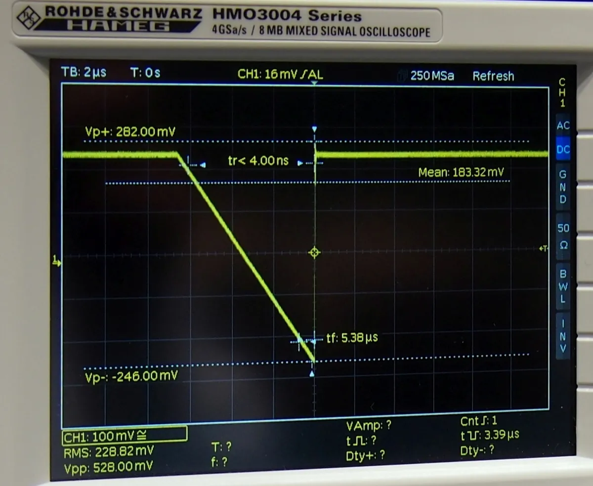
- Lab instruments: modern oscilloscopes measure rise and fall times automatically.
- Electronics design: data converters and amplifiers are specified by their settling time to a given error band.
- Robot joints: a step test on each joint is a quick health check after maintenance.
- Spec sheets: when you buy a sensor or actuator, its response time is a step-response number — check how it was defined.
Bench build
Bench build: record a real step response
No controller this time — we measure the *plant*. step_logger.ino holds the LED dim for 2 s, then steps it bright and records the LDR reading every 2 ms for 0.6 s. It prints the data as CSV and computes rise time, overshoot and settling time on the board. Each analogRead() returns a 10-bit value (0–1023) on an UNO. Want to know how long one read takes? Time it with micros() — it is a good habit before choosing a sample period.
Same wiring
Pin 9 → 220 Ω → LED → GND; 5 V → LDR → A0 → 10 kΩ → GND; paper tube around both.
Upload and open Serial Monitor
115200 baud. Every few seconds a new block of
t_ms,readinglines appears, followed by a#summary line.Plot it
Copy one block into a spreadsheet and draw a line chart. Mark the 10 % and 90 % points by hand.
Compare
Check the board’s rise time against your hand measurement and against
metrics()in Python.Change the step
Try LOW_PWM 0 → HIGH_PWM 255, and 100 → 150. Do the metrics change? (The LDR is not linear, so they may.)
// step_logger.ino - record a step response from the LED + LDR bench and measure it.
// Wiring (same as Lessons 2-8): pin 9 -> 220 ohm -> LED -> GND;  5V -> LDR -> A0 -> 10k -> GND.
// No controller here: we step the LED from LOW_PWM to HIGH_PWM and watch how the SENSOR responds.
// Copy the CSV lines from the Serial Monitor into a spreadsheet to plot them.

const int LED_PIN = 9, SENSOR_PIN = A0;
const int LOW_PWM = 40, HIGH_PWM = 200;
const int N = 300;                 // samples
const unsigned long SAMPLE_US = 2000;   // one sample every 2 ms -> 0.6 s of data
int samples[N];

void setup() {
  pinMode(LED_PIN, OUTPUT);
  Serial.begin(115200);
}

void loop() {
  analogWrite(LED_PIN, LOW_PWM);
  delay(2000);                                  // let the LDR settle at the low level

  unsigned long t0 = micros();
  analogWrite(LED_PIN, HIGH_PWM);               // the STEP
  for (int i = 0; i < N; i++) {
    while (micros() - t0 < (unsigned long)i * SAMPLE_US) { }   // fixed sample times
    samples[i] = analogRead(SENSOR_PIN);
  }

  // final value = average of the last 20 samples; start = first sample
  long sum = 0;
  for (int i = N - 20; i < N; i++) sum += samples[i];
  float finalV = sum / 20.0, startV = samples[0], span = finalV - startV;
  int i10 = -1, i90 = -1, iPeak = 0, iSettle = 0;
  for (int i = 0; i < N; i++) {
    if (i10 < 0 && samples[i] >= startV + 0.1 * span) i10 = i;
    if (i90 < 0 && samples[i] >= startV + 0.9 * span) i90 = i;
    if (samples[i] > samples[iPeak]) iPeak = i;
    if (abs(samples[i] - finalV) > 0.02 * abs(span)) iSettle = i;
  }

  Serial.println(F("t_ms,reading"));
  for (int i = 0; i < N; i++) {
    Serial.print(i * SAMPLE_US / 1000.0, 1); Serial.print(','); Serial.println(samples[i]);
  }
  Serial.print(F("# start=")); Serial.print(startV, 0);
  Serial.print(F(" final=")); Serial.print(finalV, 1);
  Serial.print(F(" rise_10_90_ms=")); Serial.print((i90 - i10) * SAMPLE_US / 1000.0, 1);
  Serial.print(F(" overshoot_pct=")); Serial.print(span != 0 ? (samples[iPeak] - finalV) / span * 100 : 0, 1);
  Serial.print(F(" settle_2pct_ms=")); Serial.println(iSettle * SAMPLE_US / 1000.0, 1);
  delay(5000);                                  // pause, then repeat the test
}Debugging
Debugging your measurements
| Symptom | Likely cause | Fix |
|---|---|---|
| Rise time is 0 or negative | Start value taken after the step began | Take the start value just before the step |
| Settling time equals the log length | Never settles in the window, or noise exceeds the band | Log longer; average; widen the band and say so |
| Overshoot shows huge % | Tiny span (final ≈ start) | Use a bigger step |
| Metrics change every run | Sensor noise or room light | Repeat 5 times and report the average |
| Board and Python disagree | Different definitions or sample times | Use the same band, same final-value method |
Think
Think about it
Think
Team A reports “overshoot 4 %, settling 0.9 s”. Team B reports “overshoot 6 %, settling 1.2 s” for an identical arm and controller. Give three reasons the numbers could differ even though the robots behave the same.
Experiment
Try it in the lab: measure, don’t guess
About 35 minutes with the response lab, the metrics function and the step logger.
Experiment
Measure, don’t guess
You will need
- Control response lab (in your browser)
- `step_metrics.py`
- Optional: Arduino UNO, LED, 220 Ω, LDR, 10 kΩ, spreadsheet
Steps
- In the response lab, pick two gain settings that “look” similar. Write down which you think is better.
- Measure both with the five metrics. Were you right?
- Run `step_metrics.py`. Repeat with a 5 % band and note what changes.
- Optional bench: record three steps with `step_logger.ino`; average their metrics.
- Write a one-paragraph “test procedure” another team could follow to get the same numbers.
Interactive · Control response lab
Goal: |SSE| ≤ 2°, overshoot ≤ 15% · Hint: Moderate Kp, light Kd, tiny Ki
|SSE|
0.24°
Overshoot
32.7%
Result
RETRY
Metrics turn “fast and smooth” into numbers. They only mean something when the definitions and the test procedure are written down.
Knowledge check
Check your understanding
Knowledge check
1. Rise time is usually measured…
2. Settling time is the time until the output…
3. Percent overshoot (Control Tutorials) is measured against…
4. In the code lab, which controller had the fastest rise time?
5. PD and PID had almost the same rise, peak and settling. What did PID add?
6. Why average the last 0.2 s for the final value?
7. If you stop logging before the response settles…
8. Why does step_logger.ino wait in a loop until each sample time?
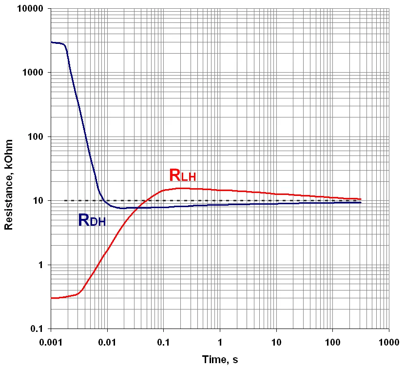
9. The vactrol chart shows an LED + LDR pair that…
10. Two teams get different metrics for identical robots. The first thing to check is…
Mini assignment
Hands-on assignment
Mini assignment
Step response report card
Create a repeatable test procedure and a report card for at least two controllers (simulated or bench).
Deliverables
- Your written test procedure: step size, sample period, log length, band, final-value method.
- A report-card table with all five metrics for at least two controllers.
- One plot per controller with rise, peak and settling marked.
- If you built it: three bench step responses and their averaged metrics.
- A short paragraph: which controller is “better” and for what kind of task?
Do this, step by step
- Write a short test procedure: step size, sample period, log length, settling band and how you take the final value.
- Run
python3 step_metrics.py, copy the report card, and check one metric by hand from the printed data. - Use
metrics()on two different controllers (e.g. two rows from Lesson 8) and fill in a report-card table with all five metrics. - In the response lab widget compare two gain settings using the numbers it shows, not the look of the curve.
- If you have the light keeper: flash
step_logger.ino(step fromLOW_PWM= 40 toHIGH_PWM= 200), record three step responses, average the metrics, and decide which controller is “better” for which task.
Stuck? Hints, one at a time
- Hint 1: Reuse
metrics()fromstep_metrics.pyon your own lists of times and values. - Hint 2: For bench CSV, read it with Python’s
csvmodule and convert to two lists. - Hint 3: If settling time equals the log length, the response did not settle — log longer.
- Hint 4: “Better” depends on the task: a pick-and-place arm may value settling; a camera gimbal may value no overshoot.
Challenges (pick by level)
- 🟢 Easy: From the code-lab table, which controller would you choose for a gentle camera arm? Why?
- 🟢 Easy: Draw a step response by hand and label all five metrics.
- 🟡 Medium: Add “time to first reach 98 %” to
metrics()and compare it with settling time. - 🟡 Medium: Run the bench logger with two step sizes and explain any difference in rise time.
- 🟠 Hard-ish: Make
metrics()work for downward steps (90° → 0°) too. - 🔴 Hard: Use the Control Tutorials’ first-order rule (time constant = time to reach 63 %) to estimate a time constant for your LDR from the bench data.
- ⚫ Research: Read the Control Tutorials’ System Analysis page and explain how damping ratio relates to percent overshoot for a second-order system.
Next step
Now that you can measure a response, you can tune it on purpose. In Lesson 10 — Tuning Intuition you learn a step-by-step way to change gains and watch the metrics move.
Look back: Lesson 8: Combining PID. Next: Lesson 10: Tuning Intuition. Related: Stage 2 — Programming & Python (plotting data) and Stage 9 — Trajectory Planning.
Sources
- Control Tutorials (University of Michigan) — Introduction: System Analysis — settling time (within e.g. 2 % of steady state), rise time (typically 10–90 %), percent overshoot relative to the final steady-state value, first-order time constant (63 %).
- Arduino Docs — analogRead() — on an UNO the analog input is read as a 10-bit value, 0–1023.
- Control Tutorials (University of Michigan) — Introduction: PID Controller Design — effects of P, I and D on rise time, overshoot, settling time and steady-state error.
- Photos and diagrams: Wikimedia Commons (credits under each image).
Self-attested for now — keep artifacts in your lab notebook.
Complete
Today's goal
0 of 1 done today
Mark this lesson complete when you have worked the experiment, knowledge check, and assignment (even roughly).