
Control Systems & PID · Lesson 06
Integral Control (I)
Est. 60–75 min
Why
Why the last few degrees need a controller with memory
In Lesson 5, P control got the joint close but left a leftover error under gravity: 5° with Kp = 0.01. The problem is simple — P only produces torque when there is an error. Integral control (I) fixes this by giving the controller a memory. It keeps adding up the error over time. As long as any error remains, the sum keeps growing, the command keeps increasing, and eventually the joint is pushed all the way to the target. When the error is zero, the sum stops changing — and *keeps* supplying exactly the torque the load needs.
By the end of this lesson you will be able to: write the PI control law; explain why the integral removes the steady-state error (Modern Robotics, Michigan Control Tutorials); run a Ki sweep and read its trade-offs — zero leftover error, but more overshoot and slower settling, and with too much Ki an oscillation that won’t die; recognise integral windup; and add a clamped integral to the LED + LDR bench loop.
Concept
How the integral term works — and what it costs
Think of a piggy bank that collects the error. Every tick, you drop in the current error (small coins for a small error, big coins for a big one; negative coins when you overshoot). The integral term pushes in proportion to how full the piggy bank is. A tiny error that stays for a long time slowly fills the bank — and that is exactly what beats a steady load like gravity.
u = Kp × e + Ki × ∫ e dt (in code: integral += e × dt; u = Kp*e + Ki*integral)
- Ki = integral gain. *Modern Robotics* (Section 11.4.1) writes the full PID law as τ = Kp θe + Ki ∫θe dt + Kd θ̇e and says the integral gain can be used to reduce or eliminate steady-state errors.
Why it removes the leftover error
*Modern Robotics* explains it neatly: with Ki > 0, the controller can produce a non-zero steady torque even with zero position error — only the *integrated* error must be non-zero. The Michigan *Control Tutorials* say the same in plain words: if there is a persistent, steady error, the integrator builds and builds, increasing the control signal and driving the error down. In our simulation, the integral term ends at about 0.05 N·m — exactly the gravity torque — and the error goes to (almost) zero.
| Ki | Final angle | Leftover error | Peak | Settles within ±2° | Integral term at end |
|---|---|---|---|---|---|
| 0 (P only) | 84.99° | 5.01° | 102.65° | never | 0 |
| 0.001 | 89.41° | 0.59° (still shrinking) | 108.24° | 3.98 s | 0.045 N·m |
| 0.002 | 90.28° | −0.28° | 113.61° | 4.93 s | 0.052 N·m |
| 0.005 | 89.99° | 0.01° | 128.18° | 5.52 s | 0.050 N·m |
| 0.02 | still swinging 4°–177° after 30 s | — | 177.00° | never | — |
The price of memory
The *Control Tutorials* warn that the integral term can make the system more sluggish and oscillatory, because when the error changes sign the integrator takes a while to “unwind”. You can see it in the table: as Ki rises, the peak climbs (108° → 128°) and settling gets slower. With Ki = 0.02 the stored error keeps flinging the joint back and forth — the loop is on the edge of instability. Their PID tutorial even lowers Kp when it adds Ki, because both push in the same direction.
| When you raise Ki… | Rise time | Overshoot | Settling time | Steady-state error |
|---|---|---|---|---|
| Effect | Decreases | Increases | Increases | Eliminated |
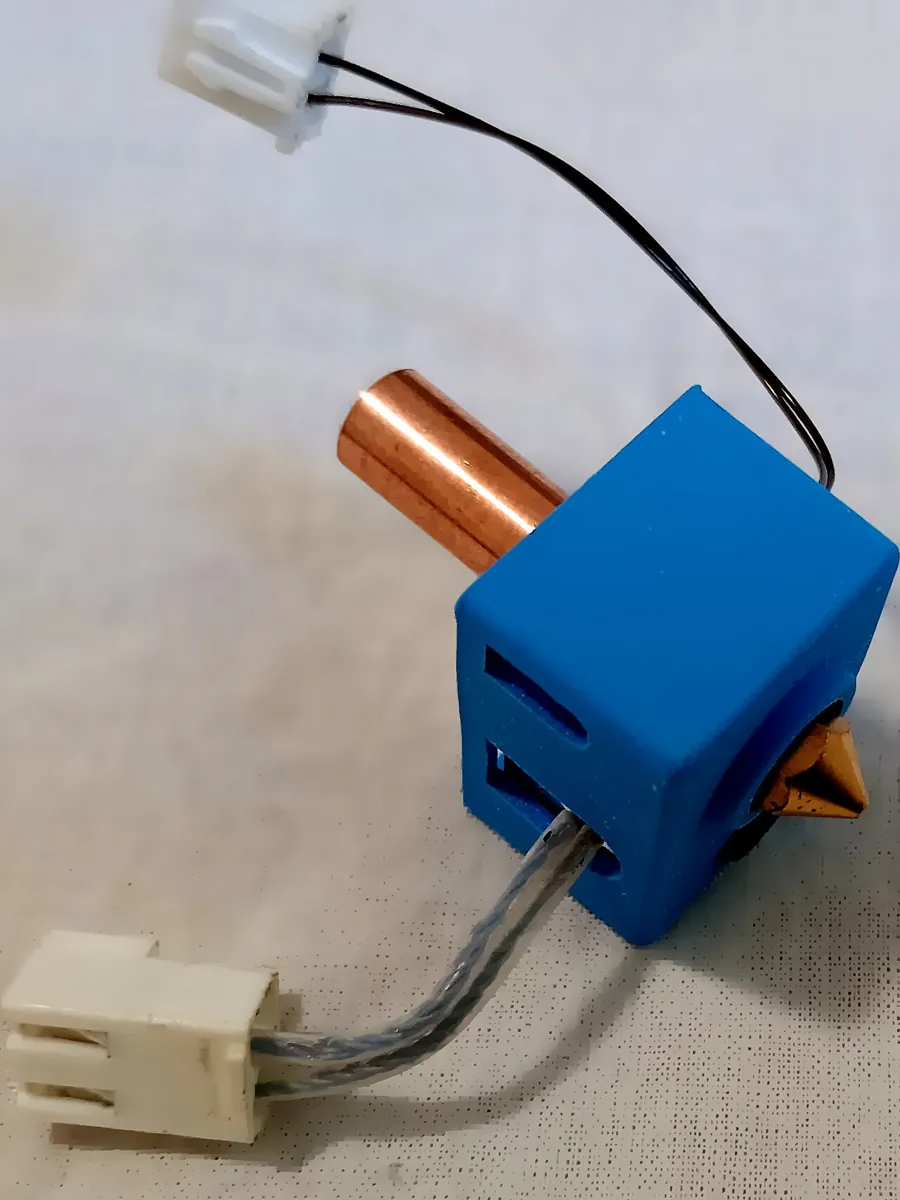
M303) that heats and cools the hot end to find good gains. The integral term is what holds the temperature exactly at, say, 210 °C instead of a few degrees below.Photo: A7N8X · CC0 · Source: Wikimedia Commons · resized, converted to WebPWindup, in one paragraph
If the actuator is already at its limit (full torque, PWM 255) and the error is still large, the integral keeps growing — but the extra command can’t do anything. When the joint finally reaches the target, the huge stored integral keeps pushing and causes a big overshoot. The simplest fix: clamp the integral to what the actuator can actually deliver, or stop integrating while the output is saturated. Both bench sketches in this stage do the first.
Visual
Visualise it: load vs Ki
Add load, then raise **Ki** step by step. The leftover error shrinks to zero — and overshoot and settling time grow. Find the smallest Ki that removes the error in a reasonable time.
Interactive · PID visualizer

Setpoint 70° · final θ 69.1° · |SSE| 0.94° · constant load on
Teaching model: Kp↑ snappier (overshoot risk); Ki↑ reduces steady-state error under load; Kd↑ damps the edge.
Code lab
Code lab: a Ki sweep on the same joint
Same joint and gravity load as Lesson 5, with Kp = 0.01 N·m/° (which left a 5° error). The script adds the integral term for five values of Ki and prints the final angle, leftover error, peak, settling time and the integral term’s final torque. Run it with python3 pi_control.py.
# pi_control.py - adding INTEGRAL action to remove the leftover (steady-state) error.
# Same joint as p_control.py: J*accel = torque - B*speed - LOAD   (angles in degrees)
# Controller (PI): torque = Kp*e + Ki * (running sum of e*dt)
J, B, LOAD, TAU_MAX = 0.002, 0.004, 0.05, 4.0
SETPOINT, DT, T_END = 90.0, 0.001, 10.0
KP = 0.01

def run(ki):
    angle = speed = integral = 0.0
    t, log = 0.0, []
    while t < T_END:
        e = SETPOINT - angle
        integral += e * DT                       # the controller's memory of past error
        torque = max(-TAU_MAX, min(TAU_MAX, KP * e + ki * integral))
        speed += (torque - B * speed - LOAD) / J * DT
        angle += speed * DT
        t += DT
        log.append((t, angle, ki * integral))
    return log

def summary(log):
    final = sum(a for _, a, _ in log[-1000:]) / 1000
    peak = max(a for _, a, _ in log)
    band = 2.0                                   # settle = stays within +/-2 deg of the setpoint
    settle = max((t for t, a, _ in log if abs(a - SETPOINT) > band), default=0.0)
    i_term = log[-1][2]
    return final, peak, settle, i_term

print(f"Kp = {KP} N.m/deg, gravity load {LOAD} N.m, setpoint {SETPOINT:.0f} deg\n")
print(f"{'Ki':>6} {'final':>8} {'SSE':>7} {'peak':>8} {'past 90°':>10} {'settle(+/-2deg)':>16} {'I-term at end':>14}")
for ki in (0.0, 0.001, 0.002, 0.005, 0.02):
    final, peak, settle, i_term = summary(run(ki))
    st = "never" if settle >= T_END - 0.01 else f"{settle:.2f} s"
    print(f"{ki:>6} {final:>7.2f}° {SETPOINT-final:>6.2f}° {peak:>7.2f}° {peak-SETPOINT:>8.2f}° {st:>15} {i_term:>11.3f} N.m")
print("\nWith Ki > 0 the integral keeps growing until it supplies the 0.05 N.m that gravity needs,")
print("so the error goes to zero. Too much Ki adds overshoot and slow wobbles -")
print("at Ki = 0.02 the joint is still swinging between about 4 and 177 deg after 30 s:")
print("the loop is on the edge of instability.")
Output (run with python3 pi_control.py)
Kp = 0.01 N.m/deg, gravity load 0.05 N.m, setpoint 90 deg

    Ki    final     SSE     peak   past 90°  settle(+/-2deg)  I-term at end
   0.0   84.99°   5.01°  102.65°    12.65°           never       0.000 N.m
 0.001   89.41°   0.59°  108.24°    18.24°          3.98 s       0.045 N.m
 0.002   90.28°  -0.28°  113.61°    23.61°          4.93 s       0.052 N.m
 0.005   89.99°   0.01°  128.18°    38.18°          5.52 s       0.050 N.m
  0.02  140.30° -50.30°  177.00°    87.00°           never      -0.218 N.m

With Ki > 0 the integral keeps growing until it supplies the 0.05 N.m that gravity needs,
so the error goes to zero. Too much Ki adds overshoot and slow wobbles -
at Ki = 0.02 the joint is still swinging between about 4 and 177 deg after 30 s:
the loop is on the edge of instability.Try it: start with a P-only response that sits below the setpoint, then raise Ki slowly. Watch the leftover error vanish — and the overshoot grow.
Interactive · PID visualizer
Setpoint 70° · final θ 69.1° · |SSE| 0.94° · constant load on
Teaching model: Kp↑ snappier (overshoot risk); Ki↑ reduces steady-state error under load; Kd↑ damps the edge.
Real world
Integral action in machines you know
- 3D printers: Marlin firmware holds hot-end and bed temperatures with PID and can autotune the gains (
M303). - Robot joints: *Modern Robotics* shows that adding Ki to PD control removes the gravity-induced error.
- Cruise control on a long hill: a pure P controller would settle a little slow; integral action brings the speed back to the set value.
- Lab ovens and water baths: PID temperature controllers hold a setpoint despite heat losses.
Bench build
Bench build: PI on the light keeper
Same LED + LDR circuit. pi_light.ino adds a clamped integral to the P controller from Lesson 5. In the Serial Plotter you will see the P term shrink and the I term grow until the reading sits right on the setpoint — even when you shade the sensor halfway.
Same wiring
Pin 9 → 220 Ω → LED → GND; 5 V → LDR → A0 → 10 kΩ → GND; paper tube around both.
Upload with KI = 1.0
Open Serial Plotter at 115200. Watch error, p_term and i_term.
Shade halfway
Hold a card to shade half the sensor for 10 s. With P only (Lesson 5) a new error remained; now the I term rises until the error is back to zero.
Sweep KI
Try 0.3, 1.0, 3.0 and 10. Note how fast the error goes to zero and whether the brightness overshoots or wobbles.
See windup
Cover the sensor completely for 10 s (the setpoint becomes unreachable, PWM hits 255). Uncover it. Note the overshoot. Then change the clamp to 0–400 and repeat — worse!
// pi_light.ino - PROPORTIONAL + INTEGRAL control on the LED + LDR light keeper.
// The integral adds up the error over time, so even a small steady error keeps pushing
// until it is gone. The integral is clamped so it cannot "wind up" beyond what the LED can do.
// Wiring: pin 9 -> 220 ohm -> LED -> GND;  5V -> LDR -> A0 -> 10k -> GND.
const int LED_PIN = 9;
const int SENSOR_PIN = A0;
const int SETPOINT = 600;
const float KP = 0.2;          // PWM per count
const float KI = 1.0;          // PWM per (count x second)
const float DT = 0.02;         // 50 Hz loop -> 0.02 s
float integral = 0;            // in PWM units after multiplying by KI
unsigned long lastTick = 0;

void setup() {
  pinMode(LED_PIN, OUTPUT);
  Serial.begin(115200);
  Serial.println(F("setpoint,reading,error,p_term,i_term,pwm"));
}

void loop() {
  if (millis() - lastTick < 20) return;
  lastTick = millis();
  int reading = analogRead(SENSOR_PIN);
  int error = SETPOINT - reading;

  integral += KI * error * DT;                // remember past error
  integral = constrain(integral, 0, 255);     // simple anti-windup clamp (Lesson 11)
  float pTerm = KP * error;
  int pwm = constrain((int)(pTerm + integral), 0, 255);
  analogWrite(LED_PIN, pwm);

  Serial.print(SETPOINT); Serial.print(',');
  Serial.print(reading);  Serial.print(',');
  Serial.print(error);    Serial.print(',');
  Serial.print(pTerm, 1); Serial.print(',');
  Serial.print(integral, 1); Serial.print(',');
  Serial.println(pwm);
}Debugging
Debugging the integral term
| Symptom | Likely cause | Fix |
|---|---|---|
| Leftover error still there | Ki too small, or integral clamped too tightly | Raise Ki; check the clamp covers the needed command |
| Slow, rolling overshoot after each move | Ki too large | Halve Ki; maybe raise Kp a little |
| Huge overshoot after being stuck at the limit | Integral windup | Clamp the integral; stop integrating while saturated |
| Behaviour changes when you change loop speed | Integral without * dt | Multiply by the real time step |
| Joint creeps slowly at rest | Integral of a small sensor offset | Calibrate the sensor; small dead band on the integral |
| Sudden jump when you change setpoint | Large old integral | Reset or limit the integral when the setpoint changes a lot |
Think
Think about it
Think
Arjun adds an integral term to his arm’s shoulder joint. It removes the sag perfectly. But when he holds the arm with his hand for 5 seconds and then lets go, the arm shoots up far past the target before coming back. Explain what happened and give two fixes.
Experiment
Try it in the lab: remove the leftover error
About 35 minutes with the visualiser, the Ki sweep and the PI light keeper.
Experiment
Remove the leftover error
You will need
- PID visualiser (in your browser)
- Your Lesson 5 P-sweep plot
- Optional: `pi_control.py`; Arduino UNO, LED, 220 Ω, LDR, 10 kΩ
Steps
- In the visualiser, set a P-only response with a visible leftover error. Raise Ki in small steps; sketch three responses.
- Run `pi_control.py`. Add the leftover error for each Ki to your Lesson 5 plot.
- Find the Ki that removes the error fastest without the peak going above 115°.
- Clamp the integral and rerun Ki = 0.02. Describe the change.
- Optional bench: run `pi_light.ino`, shade the sensor halfway, and compare with `p_light.ino`. Then try the windup test.
Interactive · PID visualizer
Setpoint 70° · final θ 69.1° · |SSE| 0.94° · constant load on
Teaching model: Kp↑ snappier (overshoot risk); Ki↑ reduces steady-state error under load; Kd↑ damps the edge.
The integral term removes the steady error that P alone cannot. It costs some overshoot and settling time, and it must be protected against windup.
Knowledge check
Check your understanding
Knowledge check
1. Integral action mainly targets…
2. In code, the integral is usually updated as…
3. Modern Robotics: with Ki > 0, a joint can hold a non-zero torque…
4. In the code lab, the integral term ends at about 0.05 N·m because…
5. A typical side effect of raising Ki is…
6. Why do the Control Tutorials reduce Kp when they add Ki?
7. Integral windup happens when…
8. The simplest windup protection used in this stage’s sketches is…
9. If your temperature probe reads 2 °C low, a PI controller will…
10. Which firmware command autotunes a 3D printer hot end’s PID?
Mini assignment
Hands-on assignment
Mini assignment
Load vs Ki report
Show how the integral term removes the leftover error, what it costs, and how you would protect it from windup.
Deliverables
- Your Lesson 5 plot extended with the PI results: leftover error and peak for at least four Ki values.
- Your chosen Kp and Ki for this joint, with one paragraph on the trade-off.
- Results of the clamped-integral experiment with Ki = 0.02.
- If you built it: plotter screenshots (or sketches) of `pi_light.ino` during the half-shade test and the windup test.
- A three-line “I note” for your future self: when to add I, how much, and how to protect it.
Do this, step by step
- Run
python3 pi_control.pyand copy the Ki sweep; add the results to your Lesson 5 plot. - Pick the Ki that removes the leftover error with the least extra overshoot and write down Kp and Ki.
- Run the clamped-integral experiment with Ki = 0.02 and compare the peak with and without the clamp.
- In the PID visualiser start from a P-only response that sits below the setpoint, then raise Ki slowly and note when the error disappears and when overshoot grows.
- If you have the light keeper: flash
pi_light.ino(KI= 1.0), shade the LDR halfway and save a plotter sketch; then cover it fully for 10 s, uncover it, and sketch the windup overshoot. Write your three-line “I note”.
Stuck? Hints, one at a time
- Hint 1: Change only
kivalues; keepKP = 0.01for a fair comparison. - Hint 2: The integral term at the end should be close to
LOADfor every Ki that works. - Hint 3: For the clamp, the needed torque is 0.05 N·m, so the integral (in °·s) must reach 0.05 ÷ Ki.
- Hint 4: In the bench windup test, uncover the sensor at the same moment each time so runs are comparable.
Challenges (pick by level)
- 🟢 Easy: Ki = 0.004. Roughly what integral (in °·s) is needed to supply 0.05 N·m?
- 🟢 Easy: Name two machines at home or school that must hold a value exactly despite a steady load.
- 🟡 Medium: Implement “conditional integration” in
pi_control.py: don’t add to the integral while the torque is atTAU_MAX. Compare with a plain clamp. - 🟡 Medium: Add a sudden extra load at t = 5 s (LOAD becomes 0.08). How fast does each Ki recover?
- 🟠 Hard-ish: Make the sensor read 1° low. Show that PI holds the *measured* angle at 90° and the real one at 91°.
- 🔴 Hard: Find, by search in code, the largest Ki that keeps the peak under 110° for Kp = 0.01, 0.02 and 0.04. Plot the boundary.
- ⚫ Research: Read the Marlin docs on M303 and PID temperature control, and explain in your own words what autotune is measuring.
Next step
Integral and high Kp both add overshoot. In Lesson 7 — Derivative Control (D) you add a virtual damper that brakes the joint as it rushes toward the target — and you meet its weakness: noise.
Look back: Lesson 5: Proportional Control (P). Next: Lesson 7: Derivative Control (D). Related: Stage 1 — Math for Robotics (rates and areas) and Stage 5 L08: Feedback & Closed-Loop Control.
Sources
- Modern Robotics — K. M. Lynch & F. C. Park (preprint PDF) — Sec. 11.4.1: PID law τ = Kp θe + Ki∫θe dt + Kd θ̇e; the integral gain reduces or eliminates steady-state errors; with Ki > 0 a non-zero steady torque is possible with zero position error.
- Control Tutorials (University of Michigan) — Introduction: PID Controller Design — a persistent error makes the integrator build and drive the error down; drawback: more sluggish and oscillatory, slow to “unwind” when the error changes sign; Kp reduced when Ki is added (double effect); effect table for Ki.
- Marlin Firmware — M303: PID autotune — heats and cools the hot end or bed to determine PID values.
- Photos: Wikimedia Commons (credits under each image).
Self-attested for now — keep artifacts in your lab notebook.
Complete
Today's goal
0 of 1 done today
Mark this lesson complete when you have worked the experiment, knowledge check, and assignment (even roughly).