
Control Systems & PID · Lesson 04
Control Loop Anatomy
Est. 55–70 min
Why
Why you must be able to name every block
So far you have used words like setpoint, error and controller. Now we put the whole loop on the table, block by block, the way control engineers draw it. Once you can name each block and the signal on each arrow, debugging becomes a hunt along a chain instead of guesswork: “Is the sensor right? Is the error right? Is the command right? Did the actuator obey? Did the plant respond?”
By the end of this lesson you will be able to: draw a feedback loop with reference, comparator, controller, actuator, plant, sensor and disturbance; name the signal on each arrow (r, e, u, y); explain inner and outer loops in a robot joint; write a fixed-rate control loop in Arduino code; and show with a simulation why a slow loop rate causes overshoot even with the same gain.
Concept
The blocks of a feedback loop, one by one
Think of a pressure cooker on the stove. You want the right pressure (the reference). The weight on the vent effectively compares the pressure with its setting (comparator and controller in one). The flame and vessel are the actuator and plant. The whistle tells you what is happening (a crude sensor for you). And opening a window, a gust of wind on the flame or adding cold water are disturbances. Every loop has the same parts — only the materials change.
The seven blocks and four signals
| Block / signal | Symbol | Job | Robot-joint example |
|---|---|---|---|
| Reference (setpoint) | r | What you want | Desired angle 60° from the trajectory planner |
| Comparator (summing junction) | e = r − y | Subtracts measurement from reference | One line of code: error = ref - measured |
| Controller | u = f(e) | Turns error into a command | P, PI or PID in the microcontroller |
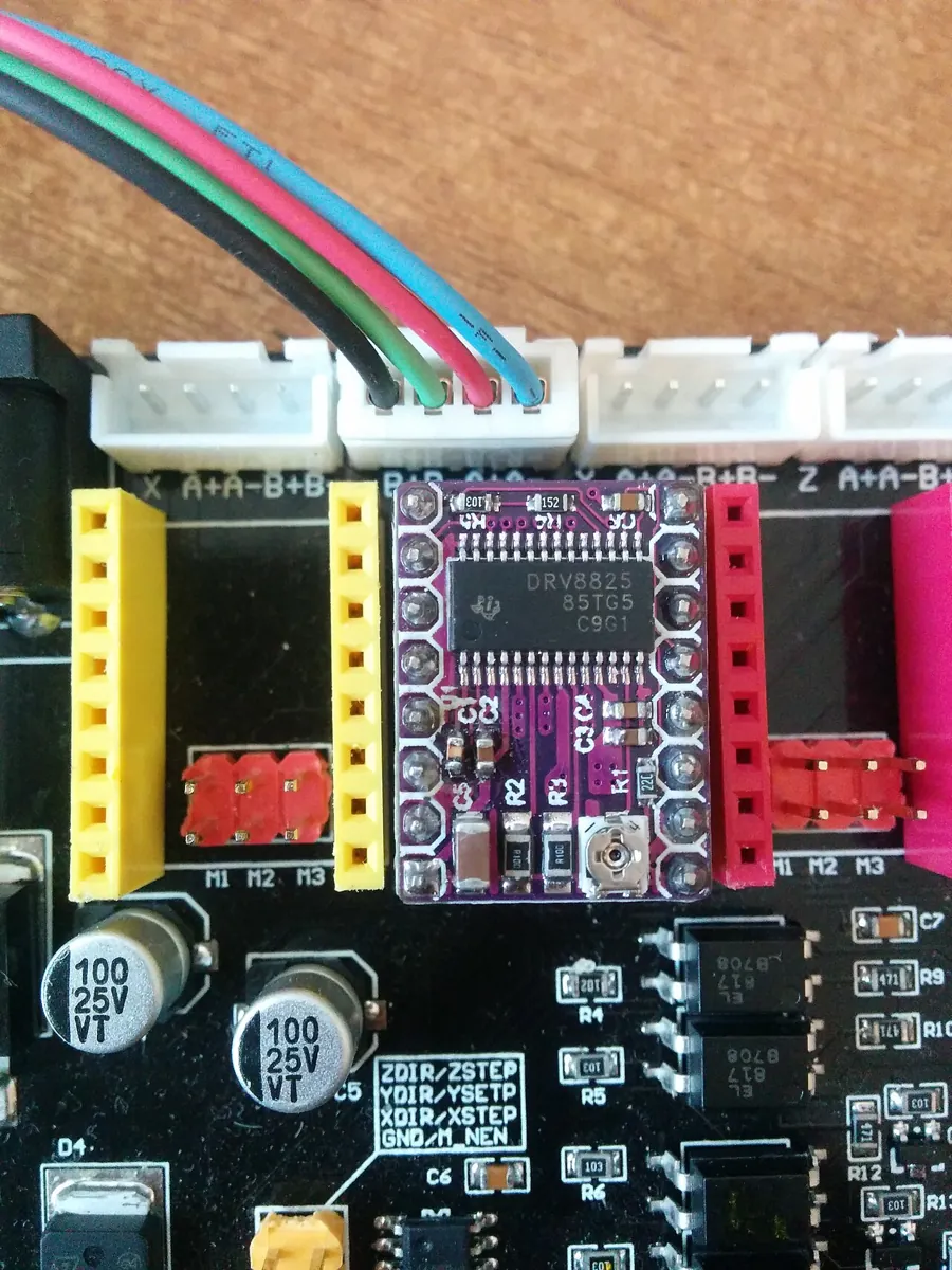
| Actuator | — | Turns the command into force or motion | Motor driver + motor + gearbox |
| Plant | — | The thing being controlled | The arm link and its load |
| Sensor (feedback path) | y | Measures the output | Encoder or potentiometer |
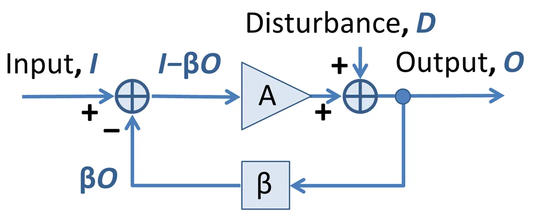
| Disturbance | d | Anything that pushes the plant off course | Gravity, friction, a bump |
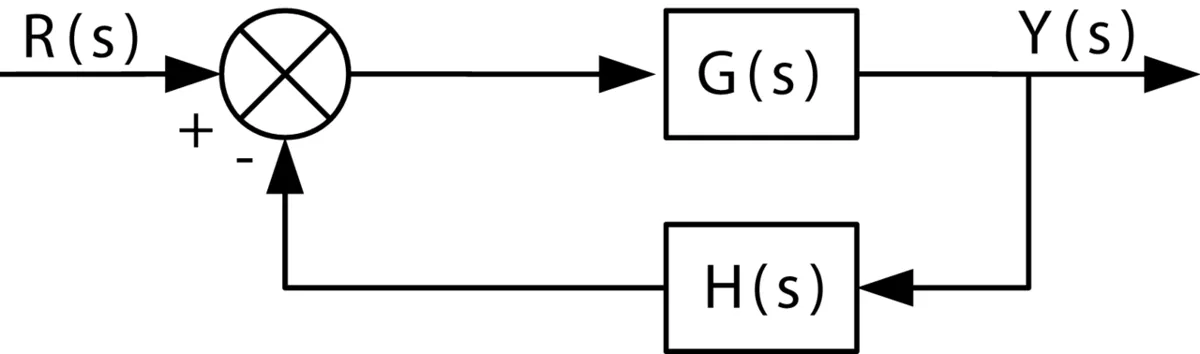
The Michigan *Control Tutorials* describe exactly this “unity-feedback” loop: the error e — the difference between desired and actual output — is fed to the controller; the controller’s signal u goes to the plant; the new output y is fed back and compared with the reference to find a new error; and the process continues while the controller is running.
Inner and outer loops
*Modern Robotics* (Figure 11.1) points out that a typical robot control system has more than one loop. The outer loop controls position. Inside it, the motor amplifier often runs its own inner loop — for example, a DC motor amplifier in torque mode senses the current actually flowing through the motor and corrects it, because motor current is proportional to torque. The outer loop says “I need this much torque”; the inner loop makes sure the motor really delivers it. The book also notes that disturbance forces can be injected before or after the arm’s dynamics.
| Loop | Measures | Commands | Typical job |
|---|---|---|---|
| Outer: position | Joint angle (encoder) | Speed or torque | Reach 60° and hold it |
| Middle: speed (sometimes) | Joint speed | Torque / current | Move smoothly at the planned speed |
| Inner: current | Motor current | Voltage (PWM) | Deliver the requested torque |
Loop rate: how often the message goes round
A controller only sees the world when it samples the sensor. Between samples it is blind and keeps sending the old command. If the loop runs too slowly, the plant moves a long way on a stale command — just like the bucket chain overfilling the tank. The code lab shows it with numbers: the same gain gives no overshoot at 100 Hz, about 1° at 20 Hz and over 6° at 5 Hz. In code, that means: run the loop at a fixed rate using millis() or micros(), and keep slow things like Serial.print out of every tick.
loop period T = 1 ÷ loop rate e.g. 100 Hz → T = 10 ms
- The loop must run fast compared with how quickly the plant moves. In the code lab, a joint that settles in well under a second behaves well at 100 Hz and poorly at 5 Hz. Current loops need far faster rates and normally live inside the motor driver.
Visual
Visualise it: trace the signal around the loop
Follow the signal around the loop: **reference → comparator → controller → actuator → plant → sensor → back to the comparator**. Add a disturbance and watch where it enters and how the loop answers.
Interactive · Control loop explorer

Mode
Closed
θ final
61.6°
Error
-1.6°
Closed-loop uses error = setpoint − feedback. Open-loop ignores feedback — load disturbances leave steady-state error.
Code lab
Code lab: a loop built from labelled blocks
The script writes each block as its own line — sensor, comparator, controller, actuator limit, plant — prints the first six ticks, then runs the same loop at 100 Hz, 20 Hz and 5 Hz. The plant has a little motor lag and a small gravity load. Run it with python3 loop_anatomy.py.
# loop_anatomy.py - one control loop, built block by block, printed tick by tick.
# reference -> [compare] -> error -> [controller] -> command -> [actuator limit] -> [plant] -> output
#                 ^                                                                       |
#                 +------------------------- [sensor] <-----------------------------------+
# Plant: a joint whose speed follows the command with a little lag; a load pushes back.
# Then we run the SAME loop at 100 Hz, 20 Hz and 5 Hz to see why loop rate matters.

def make_loop(rate_hz, kp=8.0, verbose=False):
    dt_ctrl = 1.0 / rate_hz
    dt_sim = 0.001                        # the physical world runs "continuously" (1 ms steps)
    reference, angle, speed = 60.0, 0.0, 0.0
    LOAD = -5.0                           # deg/s of drag from gravity
    TAU = 0.05                            # s, motor speed lag
    MAX_CMD = 120.0                       # deg/s actuator limit
    command, next_ctrl, t = 0.0, 0.0, 0.0
    peak, rows = 0.0, []
    while t < 2.0:
        if t >= next_ctrl - 1e-12:        # ---- one control tick ----
            measured = round(angle, 1)                 # SENSOR (0.1 deg resolution)
            error = reference - measured               # COMPARATOR
            raw = kp * error                           # CONTROLLER (P)
            command = max(-MAX_CMD, min(MAX_CMD, raw)) # ACTUATOR limit
            if verbose and len(rows) < 6:
                rows.append((t, reference, measured, error, raw, command))
            next_ctrl += dt_ctrl
        # PLANT: speed lags behind the command, load drags it, angle integrates speed
        speed += (command - speed) / TAU * dt_sim
        angle += (speed + LOAD) * dt_sim
        peak = max(peak, angle)
        t += dt_sim
    return angle, peak, rows

final, peak, rows = make_loop(100, verbose=True)
print("First six ticks at 100 Hz (every 10 ms):")
print(f"{'t (s)':>6} {'ref':>5} {'meas':>6} {'error':>6} {'Kp*e':>7} {'cmd':>6}")
for r in rows:
    print(f"{r[0]:6.2f} {r[1]:5.0f} {r[2]:6.1f} {r[3]:6.1f} {r[4]:7.1f} {r[5]:6.1f}")
print("(cmd is clipped to 120 deg/s by the actuator limit at first)\n")

print("Same loop, same gain, different loop rates:")
for hz in (100, 20, 5):
    final, peak, _ = make_loop(hz)
    print(f"  {hz:>3} Hz: final {final:6.2f} deg, peak {peak:6.2f} deg, overshoot {max(0, peak-60):5.2f} deg")
print("\nSlower loops see the error later, so they react late and overshoot more.")
Output (run with python3 loop_anatomy.py)
First six ticks at 100 Hz (every 10 ms):
 t (s)   ref   meas  error    Kp*e    cmd
  0.00    60    0.0   60.0   480.0  120.0
  0.01    60    0.1   59.9   479.2  120.0
  0.02    60    0.3   59.7   477.6  120.0
  0.03    60    0.8   59.2   473.6  120.0
  0.04    60    1.3   58.7   469.6  120.0
  0.05    60    2.0   58.0   464.0  120.0
(cmd is clipped to 120 deg/s by the actuator limit at first)

Same loop, same gain, different loop rates:
  100 Hz: final  59.35 deg, peak  59.88 deg, overshoot  0.00 deg
   20 Hz: final  59.37 deg, peak  60.96 deg, overshoot  0.96 deg
    5 Hz: final  59.34 deg, peak  66.42 deg, overshoot  6.42 deg

Slower loops see the error later, so they react late and overshoot more.Try it: change the loop rate and see how late the controller reacts. Find the slowest rate that still feels smooth.
Interactive · Loop timing budget
Wanted rate
50 Hz
Time used / loop
35.25 ms
CPU budget used
176 %
Actual rate
28.4 Hz
Serial time here = characters × 10 bits ÷ baud. On an Arduino Uno, Serial.print() returns at once while its small transmit buffer (64 bytes) has room; when you print more than the line can carry, print() waits — so in steady state each loop pays roughly this time.
Real world
Loop anatomy in real hardware
- Hobby servo: reference = pulse width, sensor = internal potentiometer, controller + actuator = the servo’s board, motor and gears (SparkFun).
- Industrial joint: outer position loop on an encoder; inner current loop in the amplifier (Modern Robotics, Fig. 11.1).
- Cruise control: reference = set speed, sensor = vehicle speed, actuator = throttle and engine, disturbance = hills and wind (Michigan Control Tutorials).
- Your bench: reference = SETPOINT, sensor = LDR, actuator = LED, plant = the light path, disturbance = your hand.
Bench build
Bench build: a fixed-rate loop with every block labelled
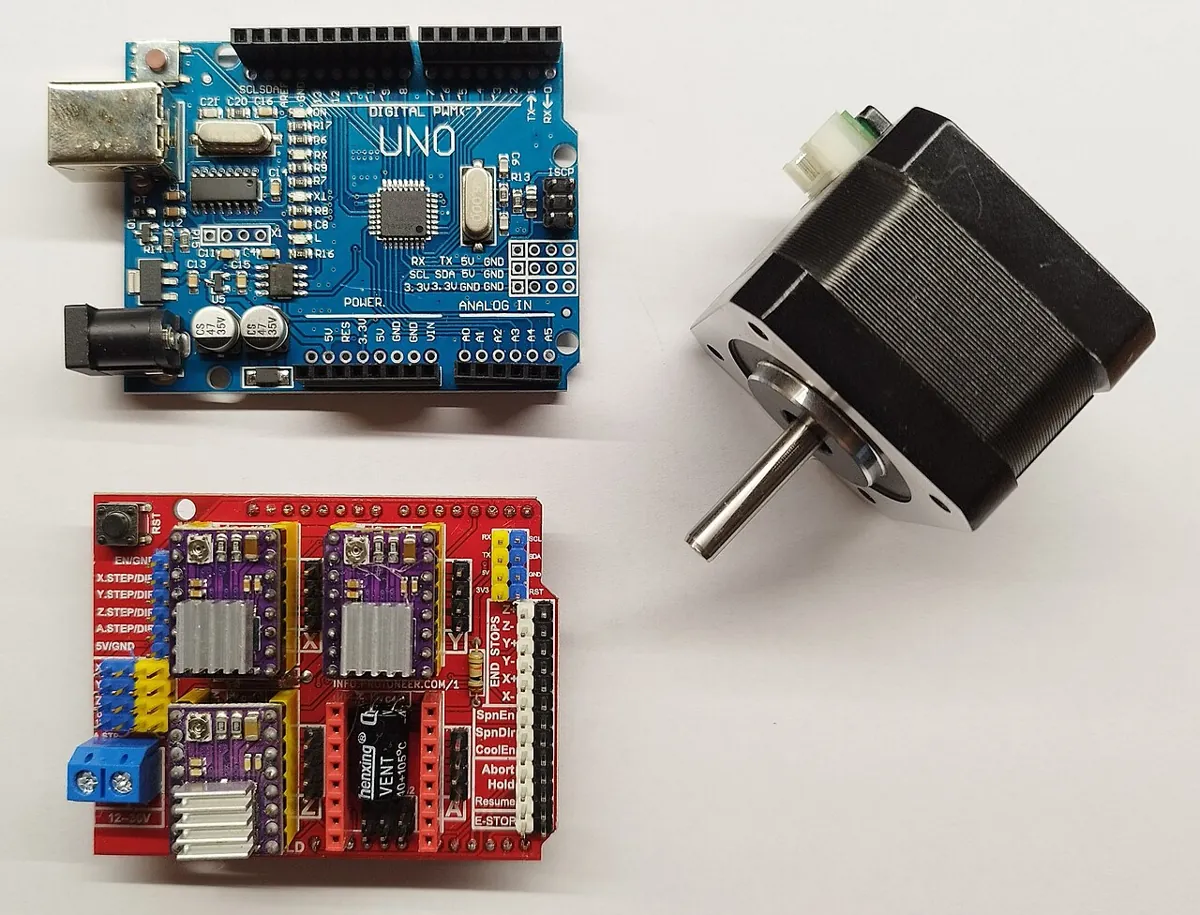
Same LED + LDR circuit as Lesson 2, but the code is split into sensorBlock(), comparatorBlock(), controllerBlock() and actuatorBlock(), and the loop runs at a fixed rate set by LOOP_HZ. Cover the sensor and watch how quickly it recovers at 100, 20 and 5 Hz.
Reuse the circuit
Pin 9 → 220 Ω → LED → GND. 5 V → LDR → A0 → 10 kΩ → GND. LED pointing at the LDR, paper tube around both.
Label your breadboard
Stick small paper tags: SENSOR (LDR), ACTUATOR (LED), PLANT (the light path), CONTROLLER (Arduino). Saying the names aloud helps.
Upload at 50 Hz
Upload
loop_anatomy.inoand open the Serial Plotter at 115200. Cover and uncover the sensor.Change the loop rate
Set
LOOP_HZto 100, then 20, then 5. For each, cover the sensor for 3 s and count roughly how long it takes to settle after you uncover it.Find the bottleneck
Change the print to every tick (
n % 1) at 100 Hz. Does the loop still keep its rate? Printmicros()differences to check.
// loop_anatomy.ino - the same light-keeping loop as light_keeper.ino, written block by block
// with a FIXED loop rate. Change LOOP_HZ (100, 20, 5) and watch how fast it settles after you
// cover the sensor. Wiring: pin 9 -> 220 ohm -> LED -> GND;  5V -> LDR -> A0 -> 10k -> GND.
const int LED_PIN = 9;
const int SENSOR_PIN = A0;
const int LOOP_HZ = 50;
const unsigned long PERIOD_US = 1000000UL / LOOP_HZ;

int reference = 600;          // REFERENCE (setpoint), counts 0..1023
const float KI_STEP = 0.05;   // controller: nudge output by KI_STEP * error each tick
float output = 0;             // controller memory
unsigned long nextTick = 0;

int sensorBlock()            { return analogRead(SENSOR_PIN); }
int comparatorBlock(int r, int y) { return r - y; }
float controllerBlock(int e) { output = constrain(output + KI_STEP * e, 0, 255); return output; }
void actuatorBlock(float u)  { analogWrite(LED_PIN, (int)u); }

void setup() {
  pinMode(LED_PIN, OUTPUT);
  Serial.begin(115200);
  Serial.println(F("ms,reference,measured,error,command"));
  nextTick = micros();
}

void loop() {
  if ((long)(micros() - nextTick) < 0) return;   // wait for the next tick
  nextTick += PERIOD_US;

  int y = sensorBlock();                 // SENSOR
  int e = comparatorBlock(reference, y); // COMPARATOR
  float u = controllerBlock(e);          // CONTROLLER
  actuatorBlock(u);                      // ACTUATOR -> PLANT (LED + air + LDR) -> SENSOR

  static int n = 0;
  if (++n % 5 == 0) {                    // print every 5th tick so Serial does not slow the loop
    Serial.print(millis()); Serial.print(',');
    Serial.print(reference); Serial.print(',');
    Serial.print(y); Serial.print(',');
    Serial.print(e); Serial.print(',');
    Serial.println((int)u);
  }
}Debugging
Debugging along the chain
| Check this block | Question to ask | How to test |
|---|---|---|
| Reference | Is the setpoint what I think, in the right units? | Print it |
| Sensor | Does the measurement match reality? | Compare with a protractor / meter |
| Comparator | Is the sign right (r − y)? | Move the plant below the setpoint; error must be positive |
| Controller | Is the command sensible for this error? | Print e and u together |
| Actuator | Does the motor/LED actually follow the command? | Run the actuator open loop with fixed commands |
| Plant | Is something mechanical blocking or slipping? | Move it by hand with power off |
| Loop rate | Is the loop running as fast as I think? | Print the time between ticks |
Think
Think about it
Think
Meera’s light keeper works perfectly at 50 Hz. She adds a long `Serial.println` of ten values every tick at 9600 baud, and now the brightness overshoots and wobbles after she uncovers the sensor. Nothing else changed. Which block or property of the loop did she break, and how should she fix it?
Experiment
Try it in the lab: label the blocks
About 30 minutes with the explorer, the script and the LED + LDR loop.
Experiment
Label the blocks
You will need
- Control loop explorer (in your browser)
- Loop timing lab (in your browser)
- Notebook
- Optional: `loop_anatomy.py`; Arduino UNO, LED, 220 Ω, LDR, 10 kΩ
Steps
- In the explorer, point to each block and say its name and the signal leaving it.
- Run `loop_anatomy.py`. For the first tick, write r, y, e, Kp·e and the clipped command.
- Record final angle and peak for 100, 20 and 5 Hz. Make a small table.
- In the loop timing lab, find the slowest rate that still feels smooth.
- Optional bench: run `loop_anatomy.ino` at 100, 20 and 5 Hz and note roughly how long it takes to settle after you uncover the sensor.
Interactive · Control loop explorer
Mode
Closed
θ final
61.6°
Error
-1.6°
Closed-loop uses error = setpoint − feedback. Open-loop ignores feedback — load disturbances leave steady-state error.
Every loop has the same skeleton. When you can name each block and signal, and you know the loop rate, you can find almost any fault by walking around the diagram.
Knowledge check
Check your understanding
Knowledge check
1. The sensor in a joint loop measures…
2. The comparator (summing junction) computes…
3. In a robot joint, the plant is…
4. Why does feedback reject a disturbance added after the forward block?
5. Modern Robotics describes an inner loop in the motor amplifier that often controls…
6. In the code lab, the same gain gives more overshoot at 5 Hz because…
7. A 100 Hz loop has a period of…
8. In the first tick of the code lab, Kp × e = 480 °/s but the command is 120 °/s because…
9. The best way to keep a steady loop rate on an Arduino is…
10. When a loop misbehaves, a good first debugging step is…
Mini assignment
Hands-on assignment
Mini assignment
Anatomy sketch of your own loop
Draw, label and measure a complete feedback loop — your bench light keeper or a robot joint — including its loop rate.
Deliverables
- A clean block diagram with all seven blocks and the four signals (r, e, u, y) labelled with real names and units from your loop.
- The table of final angle and peak at 100, 20 and 5 Hz from `loop_anatomy.py`, plus one more rate of your choice.
- If you built it: your measured loop period with and without printing every tick (use `micros()`).
- A short nested-loop diagram for one joint of the 6DOF arm: which sensors and which inner loops would you expect?
- A five-line “walk the loop” checklist you will use to debug future loops.
Do this, step by step
- Draw your loop with all seven blocks (reference, comparator, controller, actuator, plant, sensor, disturbance) and label r, e, u and y with real names and units.
- Run
python3 loop_anatomy.pyand copy the final angle and peak at 100, 20 and 5 Hz; add one more rate of your own and predict it before you run. - Use the loop-timing widget above to find the slowest rate that still feels smooth.
- If you have the light keeper: flash
loop_anatomy.ino(LOOP_HZ= 50), measure the loop period withmicros(), then print every tick and measure again. - Draw a nested-loop sketch for one 6DOF arm joint and write your five-line “walk the loop” checklist.
Stuck? Hints, one at a time
- Hint 1: Draw the plant first in the middle, then the actuator arrow into it and the sensor arrow out of it.
- Hint 2: The comparator is just a circle with + for the reference and − for the measurement.
- Hint 3: The disturbance arrow points into the plant (or its output) — never into the controller.
- Hint 4: To measure the loop period, store
micros()at each tick and print the difference every 50 ticks.
Challenges (pick by level)
- 🟢 Easy: Label the seven blocks for a room AC with a thermostat.
- 🟢 Easy: What is the loop period for 250 Hz?
- 🟡 Medium: In
loop_anatomy.py, add a disturbance at t = 1 s (subtract 10° from the angle). Compare recovery at 100 Hz and 5 Hz. - 🟡 Medium: Add a sensor delay of one tick (use the previous measurement). How does overshoot change at 20 Hz?
- 🟠 Hard-ish: Turn the plant into two nested loops in Python: an inner speed loop at 1 kHz and an outer position loop at 100 Hz.
- 🔴 Hard: On the bench, measure the LED+LDR response time by stepping the PWM and timing the reading change. What loop rate does that suggest?
- ⚫ Research: Read *Modern Robotics* Figure 11.1 and its caption. Explain, in your own words, why the inner current loop must be faster than the position loop.
Next step
You know every block. In Lesson 5 — Proportional Control (P) you design the first real controller: push in proportion to the error, and discover what Kp does to speed, overshoot and leftover error.
Look back: Lesson 3: Setpoints, Sensors & Error. Next: Lesson 5: Proportional Control (P). Related: Stage 5 L07: Sense–Plan–Act Loop and Stage 10 — ROS 2 (ROS 2 control loops).
Sources
- Control Tutorials (University of Michigan) — Introduction: PID Controller Design — unity-feedback loop: the error between desired and actual output is fed to the controller, its output goes to the plant, the new output is fed back and compared with the reference, and the process repeats.
- Modern Robotics — K. M. Lynch & F. C. Park (preprint PDF) — Fig. 11.1: a typical robot control system with an inner loop in the amplifier/actuator (e.g. sensing motor current, since current is proportional to torque); disturbance forces can be injected before or after the dynamics block.
- SparkFun Learn: Hobby Servo Tutorial — the parts of a servo’s internal loop (potentiometer feedback, pulse-width command).
- Adafruit Learn: Using a Photocell — LDR with a 10 kΩ resistor as a voltage divider for an analog input.
- Photos and diagrams: Wikimedia Commons (credits under each image).
Self-attested for now — keep artifacts in your lab notebook.
Complete
Today's goal
0 of 1 done today
Mark this lesson complete when you have worked the experiment, knowledge check, and assignment (even roughly).