
Robotics Fundamentals · Lesson 08
Feedback & Closed-Loop Control
Est. 55–70 min
Why
Why a robot that never checks its work always drifts
Modern Robotics says it plainly: feedback control uses sensors to measure the robot’s actual behaviour, compares it with the desired behaviour, and changes the commands sent to the actuators — and feedback is used in nearly all robot systems. The alternative, feedforward or open-loop control, just plays the plan without looking; the book notes that position errors accumulate over time under feedforward control. Lesson 7 gave you the loop; this lesson gives the loop a goal and the habit of correcting toward it.
By the end you will be able to: draw a closed-loop block diagram (setpoint, error, controller, actuator, plant, sensor); explain open vs closed loop with examples; compute the error and a proportional (P) correction; predict P control’s leftover error under a steady disturbance; use on–off control with hysteresis like a thermostat; explain why a hobby servo is already a closed loop; and add your own feedback loop around a joint on the bench.
Concept
Open loop and closed loop in plain words
Think of riding a bicycle in a straight line. You never hold the handlebar perfectly still. You notice a small drift left, you steer a little right; a gust pushes you, you correct again. You don’t compute the whole ride in advance — you keep comparing where you are with where you want to be, and correcting. That is closed-loop control, and you have been doing it since you were six.
The block diagram
| Block | Meaning | Robot-joint example |
|---|---|---|
| Setpoint (reference) | What you want | Desired angle: 90° |
| Sensor | Measures what actually happened | Potentiometer or encoder on the joint (Lesson 6) |
| Error | Setpoint − measurement | 90° − 74° = 16° |
| Controller | Turns error into a command | P control: command = Kp × error |
| Actuator | Applies the command | Motor + gearbox (Lesson 5) |
| Plant | The thing being controlled | The arm link, with its load |
| Disturbance | Anything that pushes the plant off course | Gravity, friction, someone bumping the arm |
error e = θ_desired − θ_measured P control: ω = Kp × e
- ω = commanded joint speed; Kp = proportional gain (1/s). Modern Robotics calls this the simplest feedback controller: a correction proportional to the position error.
Open loop vs closed loop
| Open loop (feedforward) | Closed loop (feedback) | |
|---|---|---|
| Uses sensors? | No — plays the plan | Yes — measures and corrects |
| Handles disturbances? | No — errors accumulate | Yes — corrects them (mostly) |
| Cost / complexity | Lower | Higher: sensor, wiring, tuning |
| Can go unstable? | No (but can be very wrong) | Yes, if the gain is too high or the sensor lags |
| Examples | Toaster timer, stepper without encoder | Thermostat, cruise control, servo, balancing robot |
Real robots usually combine them: a feedforward command from the planned motion (“move at 45°/s”) plus a feedback correction from the error. The plan does most of the work; feedback cleans up what the plan didn’t expect. The code lab does exactly that.
P control’s leftover error
Modern Robotics shows that when a P-controlled joint has to keep up with a constant demand it cannot see, the error settles to a non-zero steady value of that demand divided by Kp. In our simulation a load slows the joint by 8°/s; with Kp = 5 the joint settles 8 ÷ 5 = 1.6° short. A bigger Kp shrinks the error, but real joints have speed limits and sensor noise, so Kp cannot grow forever. Stage 7 adds the integral term (I) that removes the leftover error.
steady error (P only) = disturbance rate ÷ Kp
- 8 °/s ÷ 5 /s = 1.6°. Double Kp → half the error.
On–off control and hysteresis
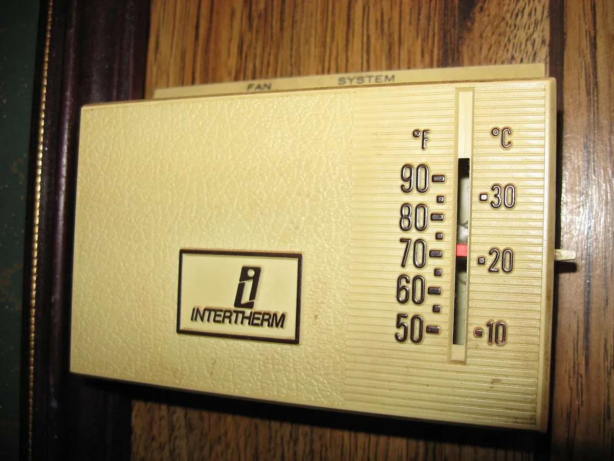
Not every loop needs smooth commands. A thermostat switches a heater fully ON below 20 °C and fully OFF above 22 °C. The gap between the two thresholds is hysteresis — it stops the heater clicking on and off every second when the temperature sits near one value. Robots use the same trick for states (Lesson 7) and for fans, pumps and grippers.
Your servo is already a closed loop
SparkFun defines a servomechanism as a device that uses feedback to achieve the desired result. Inside a hobby servo, a potentiometer measures the output shaft, the servo’s circuit compares it with the pulse width you sent, and drives the motor until they match (Adafruit describes the same parts: DC motor, gear train, H-bridge driver and potentiometer). So when you write servo.write(90), you are giving a *setpoint* to a closed loop. What you can’t do with a plain hobby servo is *see* its error — which is why the bench build adds an outside sensor.
Visual
Visualise it: close the loop
Follow the arrows around the loop: **setpoint → error → controller → actuator → plant → sensor → back to the error**. Change the setpoint or add a disturbance and watch the loop correct itself.
Interactive · Open-loop vs closed-loop
Current
20.0°
Error (seen)
40.0°
Correction
10.0
Overshoot
0.0°
Closed-loop: correction = gain × error, capped at ±12° per tick, applied every 120 ms. Open-loop holds the plant where it is — target changes do nothing without a model. Try gain 1.2 with 3 ticks of delay to see oscillation.
Code lab
Code lab: open loop vs P control, and a thermostat
The script moves a joint from 0° to 90° in 2 s, with a load that slows it by 8°/s. Open loop plays the planned speed. Closed loop adds a P correction (Kp = 5). Then a thermostat with hysteresis runs for 40 minutes. Run it with python3 open_closed.py.
"""open_closed.py - move a joint from 0 to 90 deg in 2 s.
Open loop (feedforward): send the planned velocity, never look.
Closed loop (P control, Modern Robotics 11.3): velocity = planned + Kp * (desired - measured).
A constant disturbance (gravity / friction) slows the joint by 8 deg/s."""

DT, T_END = 0.02, 3.0
DISTURB = -8.0     # deg/s pulled off every step by the load
KP = 5.0           # 1/s

def desired(t):
    return 90.0 * min(t, 2.0) / 2.0

def desired_rate(t):
    return 45.0 if t < 2.0 else 0.0

def run(closed):
    th, log = 0.0, []
    for n in range(round(T_END / DT)):
        t = n * DT
        cmd = desired_rate(t) + (KP * (desired(t) - th) if closed else 0.0)
        th += (cmd + DISTURB) * DT
        log.append((round(t + DT, 2), th))
    return log

ol, cl = run(False), run(True)
print(" t(s)  desired  open-loop  error   closed-loop  error")
for (t, a), (_, b) in zip(ol, cl):
    if abs(t * 2 - round(t * 2)) < 1e-6:
        d = desired(t)
        print(f"{t:4.1f}  {d:7.1f}  {a:9.1f}  {d-a:5.1f}   {b:10.1f}  {d-b:5.1f}")
print(f"\nfinal error: open loop {90-ol[-1][1]:.1f} deg, P control {90-cl[-1][1]:.1f} deg")
print(f"steady error with P only = disturbance / Kp = {-DISTURB/KP:.1f} deg (Stage 7 adds I to remove it)")

print("\n== On-off control with hysteresis (thermostat style) ==")
temp, heater = 18.0, False
for minute in range(0, 41, 4):
    if temp < 20.0: heater = True
    if temp > 22.0: heater = False
    print(f"{minute:2d} min  {temp:4.1f} C  heater {'ON ' if heater else 'off'}")
    temp += (0.8 if heater else -0.5) * 4 / 2
Output (run with python3 open_closed.py)
 t(s)  desired  open-loop  error   closed-loop  error
 0.5     22.5       18.5    4.0         21.0    1.5
 1.0     45.0       37.0    8.0         43.4    1.6
 1.5     67.5       55.5   12.0         65.9    1.6
 2.0     90.0       74.0   16.0         88.4    1.6
 2.5     90.0       70.0   20.0         88.4    1.6
 3.0     90.0       66.0   24.0         88.4    1.6

final error: open loop 24.0 deg, P control 1.6 deg
steady error with P only = disturbance / Kp = 1.6 deg (Stage 7 adds I to remove it)

== On-off control with hysteresis (thermostat style) ==
 0 min  18.0 C  heater ON
 4 min  19.6 C  heater ON
 8 min  21.2 C  heater ON
12 min  22.8 C  heater off
16 min  21.8 C  heater off
20 min  20.8 C  heater off
24 min  19.8 C  heater ON
28 min  21.4 C  heater ON
32 min  23.0 C  heater off
36 min  22.0 C  heater off
40 min  21.0 C  heater off
Try it: keep the tank at the line by controlling the inflow. Change the gain and add a leak (a disturbance) — exactly the bucket from the story.
Interactive · Water tank: float switch vs timer
Overflow wasted
0 L
Minutes dry
0 min
Pump running
74 min
Pump switchings
4
Model: 1000 L tank, starts at 300 L, simulated minute by minute for 3 hours. Float switch = closed loop (it senses the level). Timer = open loop (it never looks at the tank).
Real world
Feedback in real machines — old and new
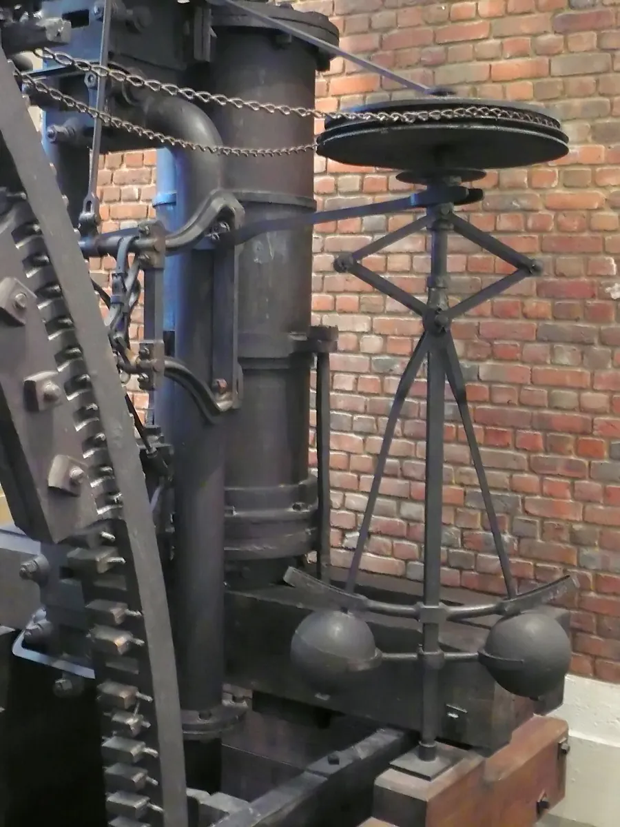
- Steam engines (1788): the centrifugal governor kept engine speed steady by closing the valve as speed rose.
- Homes: thermostats switch heating or cooling with hysteresis.
- Hobby servos: an internal potentiometer closes the position loop.
- Line-following robots: IR sensors measure how far the line is from the centre; the wheel speeds are corrected to steer back.
- Industrial arms: every joint runs fast feedback loops on its encoder; Modern Robotics: feedback is used in nearly all robot systems.
Bench build
Bench build: add your own feedback loop around a joint
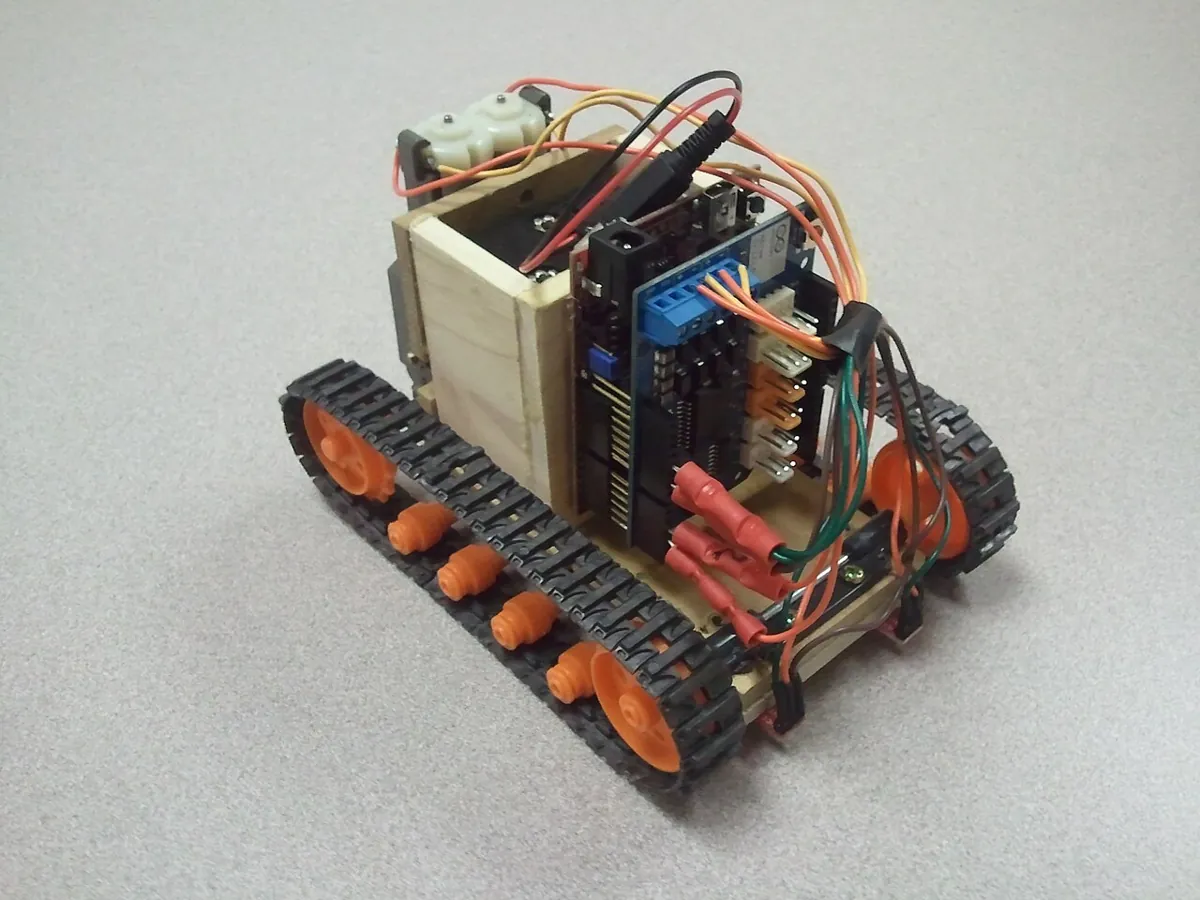
A knob sets the target angle. A second potentiometer, coupled to the servo’s horn, measures the real joint angle. The Arduino adds a P correction to the servo command. Hang a small load on the arm and compare CLOSED_LOOP = false with true.
Couple the sensor
Mount a 10 kΩ pot so its shaft turns with the servo horn (a short piece of tube or a 3D-printed coupler). This is your joint sensor from Lesson 6.
Wire the knob and sensor
Both pots: outer legs to 5 V and GND. Knob wiper → A0 (target). Joint pot wiper → A1 (measured).
Wire the servo
Signal → pin 9. Servo power from a separate 5–6 V supply; supply GND joined to Arduino GND.
Calibrate first
With
CLOSED_LOOP = false, turn the knob and compare target and measured in the Serial Monitor. AdjustpotToDeg()for each pot until they agree within a few degrees with no load.Add a load
Tape a small weight (20–30 g) near the end of the arm. Note the steady error in open loop.
Close the loop
Set
CLOSED_LOOP = trueand upload. The error should shrink. TryKP = 0.2,0.5and1.0and note error and any wobble.
// p_correct_servo.ino - add YOUR OWN feedback loop around a joint.
// A knob (pot on A0) sets the target angle. A second pot on A1 is coupled to the joint shaft
// and measures the real angle. Proportional correction: command = target + KP * (target - measured).
// Servo signal on pin 9; servo power from a separate 5-6 V supply with grounds joined.
#include <Servo.h>

Servo joint;
const float KP = 0.5;
const int SOFT_MIN = 20, SOFT_MAX = 160;
const bool CLOSED_LOOP = true;    // set false to compare open loop

float potToDeg(int counts) { return counts * 180.0 / 1023.0; }   // calibrate for your pots

void setup() {
  Serial.begin(9600);
  joint.write(90);
  joint.attach(9);
}

void loop() {
  float target = constrain(potToDeg(analogRead(A0)), SOFT_MIN, SOFT_MAX);
  float measured = potToDeg(analogRead(A1));
  float error = target - measured;
  float cmd = CLOSED_LOOP ? target + KP * error : target;
  cmd = constrain(cmd, SOFT_MIN, SOFT_MAX);
  joint.write((int)cmd);
  Serial.print("target "); Serial.print(target, 1);
  Serial.print("  measured "); Serial.print(measured, 1);
  Serial.print("  error "); Serial.println(error, 1);
  delay(20);   // 50 Hz, the same rate as the servo pulses
}Debugging
Debugging feedback loops
| Symptom | Likely cause | Fix |
|---|---|---|
| Joint runs away to an end stop | Sensor sign reversed (positive feedback) | Flip the sign of the error or swap the pot’s outer legs |
| Joint oscillates (wobbles back and forth) | Gain too high, or sensor reading lags | Lower Kp; read the sensor every loop; reduce filtering delay |
| Steady error that won’t go away | P control with a constant load | Raise Kp a little; Stage 7 adds an integral term |
| Jittery command, servo buzzes | Noisy sensor amplified by Kp | Average readings; add a small dead band around zero error |
| Thermostat clicks on/off constantly | No hysteresis | Use two thresholds |
| Closed loop worse than open loop | Sensor badly calibrated | Calibrate with a protractor first (Lesson 6) |
Think
Think about it
Think
Meera’s stepper-motor gantry (no encoder) draws perfect squares for an hour. Then a pen catches on the paper, the motor skips a few steps, and every square after that is shifted. Arjun’s servo arm, drawing the same squares, recovers after the pen catches. Explain the difference using open and closed loop — and suggest one fix for Meera.
Experiment
Try it in the lab: open loop vs closed loop
Thirty minutes with the feedback visual, the water-tank lab, the script and — if you have one — the bench loop.
Experiment
Open loop vs closed loop
You will need
- Feedback loop visual (below, runs in your browser)
- Notebook
- Optional: `open_closed.py`; Arduino, servo, two 10 kΩ pots, 5–6 V supply
Steps
- In the feedback visual, name each block aloud as you trace the loop. Add a disturbance and describe the correction.
- Run `open_closed.py`. Write the final error for open loop and for P control.
- Change `KP` to 2, 5 and 20. Make a small table of Kp vs final error. Does it match disturbance ÷ Kp?
- Run the water-tank lab with a leak. Find a gain that keeps the level close without wild swings.
- Optional bench: measure the joint error under load with the loop off and on, for three values of `KP`.
Interactive · Open-loop vs closed-loop
Current
20.0°
Error (seen)
40.0°
Correction
10.0
Overshoot
0.0°
Closed-loop: correction = gain × error, capped at ±12° per tick, applied every 120 ms. Open-loop holds the plant where it is — target changes do nothing without a model. Try gain 1.2 with 3 ticks of delay to see oscillation.
Open loop is simple but blind: disturbances add up. Closed loop measures and corrects — P control leaves a small steady error under a constant load, shrinking as Kp grows, until speed limits and noise get in the way.
Knowledge check
Check your understanding
Knowledge check
1. Feedback control means…
2. The error in a position loop is…
3. Why do errors accumulate in open-loop (feedforward) control?
4. With P control, a constant disturbance of 8 °/s and Kp = 5 /s, the steady error is about…
5. Doubling Kp (within the joint’s limits) makes the steady error…
6. A thermostat uses two thresholds (ON below 20 °C, OFF above 22 °C) to…
7. A hobby servo is a closed loop because…
8. Your new loop drives the joint straight to an end stop. Most likely…
9. The centrifugal governor on a steam engine is an example of…
10. Real robots often combine feedforward and feedback because…
Mini assignment
Hands-on assignment
Mini assignment
Prove feedback beats a plan
Show, with your own numbers, how open-loop and closed-loop control behave under a disturbance — in simulation and, if you can, on a real joint.
Deliverables
- A labelled block diagram of your bench loop (or the simulated joint) with setpoint, sensor, error, controller, actuator, plant and disturbance.
- A table of Kp vs final error from `open_closed.py`, with a line showing it matches disturbance ÷ Kp.
- If you built the bench loop: errors under load with the loop off and on for three gains, plus one sentence on any wobble you saw.
- One paragraph: name three closed loops in your home or school and identify their sensors.
Do this, step by step
- Draw the block diagram of your loop: setpoint, error, controller, actuator, plant, sensor and disturbance.
- Run
open_closed.pyand note the open-loop and closed-loop errors under the disturbance. - Change Kp to three values, record the final error for each, and check it matches disturbance ÷ Kp.
- Optional bench: flash
p_correct_servo.ino, hang a small load on the horn and record the error with the loop off and on for three gains. - Name three closed loops in your home or school and identify the sensor in each.
Stuck? Hints, one at a time
- Hint 1: For the block diagram, start with the plant (the arm) in the middle. The actuator pushes into it; the sensor reads out of it.
- Hint 2: The disturbance arrow also points into the plant — it is something you don’t control.
- Hint 3: For the table, change only
KPbetween runs and copy the “final error” line. - Hint 4: If the bench joint wobbles, halve
KP. If it runs away, flip the sign.
Challenges (pick by level)
- 🟢 Easy: Is a ceiling fan with a regulator open or closed loop? Explain.
- 🟢 Easy: Compute the P steady error for a disturbance of 12 °/s with Kp = 4.
- 🟡 Medium: Add a speed limit to
open_closed.py(clampcmdto ±60 °/s). Try Kp = 50. What changes? - 🟡 Medium: Add a dead band to
p_correct_servo.ino: ignore errors smaller than 2°. Does the buzzing stop? - 🟠 Hard-ish: Add an integral term to the script:
integral += e*DT,cmd += KI*integral. Find a KI that removes the steady error without big overshoot. - 🔴 Hard: Simulate sensor delay (use the measurement from 5 steps ago). Find the Kp where the loop starts to oscillate.
- ⚫ Expert: Read Modern Robotics Section 11.3 and derive why the P controller’s error for a constant-speed reference settles at c / Kp. Relate it to your simulation.
Next step
You can make a joint go where you want. In Lesson 9 — Workspace & Reach you find out *where* the tool can go at all: the reach ring, the dead zones, the table and the two ways an elbow can bend.
Look back: Lesson 7: Sense–Plan–Act Loop. Next: Lesson 9: Workspace & Reach. Related: Stage 7 — Control Systems & PID and Stage 4 — Electronics.
Sources
- Modern Robotics — K. M. Lynch & F. C. Park (preprint PDF) — Preface: the same principles apply to a thermostat or fly-ball governor; Sec. 11.1: feedback control uses sensors to measure actual behaviour, compares it with the desired, and modulates the actuator commands, and is used in nearly all robot systems; Sec. 11.3: feedforward / open-loop control needs no sensor data and its position errors accumulate; P control θ̇ = Kp θe; a constant-rate reference leaves a steady error c / Kp, and practical limits on Kp.
- SparkFun Learn: Hobby Servo Tutorial — a servomechanism is a device that uses feedback; the internal potentiometer provides position feedback.
- Adafruit Motor Selection Guide — an RC servo is a DC motor, gear train, H-bridge driver and potentiometer for position feedback.
- Photos: Wikimedia Commons (credits under each image).
Self-attested for now — keep artifacts in your lab notebook.
Complete
Today's goal
0 of 1 done today
Mark this lesson complete when you have worked the experiment, knowledge check, and assignment (even roughly).