
Robotics Fundamentals · Lesson 04
Configuration Space Intuition
Est. 50–65 min
Why
Why roboticists draw maps of joint angles
Lesson 3 taught you to count freedoms. This lesson turns them into a space. Modern Robotics defines a robot’s configuration as a specification of the positions of *all* points of the robot, and the configuration space (C-space) as the space of all configurations. Because links are rigid, a few numbers are enough: for an arm, just the joint angles. So for a 2-joint arm, every possible pose is one point on a 2-D map — and planning a safe motion becomes drawing a line on that map that avoids the forbidden regions.
By the end you will be able to: explain configuration and C-space in your own words; draw the C-space of a 2R arm as a grid of (θ₁, θ₂) cells; mark joint limits and obstacle regions on it; tell C-space apart from workspace (Lesson 9); explain why one pose in C-space is one exact arm shape, but one tip position can come from two different C-space points; and see why motion planners work in C-space.

Concept
Configuration space in plain words: every pose is one dot
Imagine an old radio with two knobs: one for volume, one for tuning. Every setting of the radio is one pair of knob positions, which you could mark as one dot on a square chart (volume across, tuning up). The chart is the radio’s “configuration space”. Some dots are fine; some you never want (volume at maximum at midnight — a forbidden region!). A robot arm is the same, except the knobs are joints and the forbidden regions are joint limits and collisions.
The key words
| Word | Meaning | For a 2R arm |
|---|---|---|
| Configuration | Where every point of the robot is | One pair (θ₁, θ₂) |
| C-space | The space of all configurations; its dimension = DOF | A 2-D map of all (θ₁, θ₂) pairs |
| Joint limits | Bounds on how far each joint can travel | Bands you cannot enter |
| C-space obstacle | All configurations where the robot touches an obstacle | A blob on the map |
| Free C-space | Everything left: inside limits and collision-free | Where you may plan paths |
| Workspace (Lesson 9) | Where the end-effector can reach in the real world | A ring on the table |
Modern Robotics gives a lovely fact about shape: the C-space of a 2R arm with no joint limits is a torus (the surface of a doughnut), because each angle wraps around — 360° is the same as 0°. Cut the doughnut and flatten it, and you get a square whose left edge equals its right edge and whose top equals its bottom. With joint limits, the angles no longer wrap and the C-space is just a rectangle — which is what you draw on graph paper.
dim(C-space) = number of DOF
- A door: a line segment of angles (1-D). A 2R arm: a square of angle pairs (2-D). Your 6DOF arm: a 6-D space — impossible to draw, easy to compute.
From C-space point to real-world arm shape
Given a point (θ₁, θ₂) and link lengths L₁, L₂, trigonometry from Stage 1 gives the tip position. This is forward kinematics — you will meet it properly in Stage 8, but the 2-D version is just two vectors added:
x = L₁ cos θ₁ + L₂ cos(θ₁ + θ₂), y = L₁ sin θ₁ + L₂ sin(θ₁ + θ₂)
- θ₁ = shoulder angle from the x-axis; θ₂ = elbow angle measured from the line of the upper arm.
Obstacles become blobs
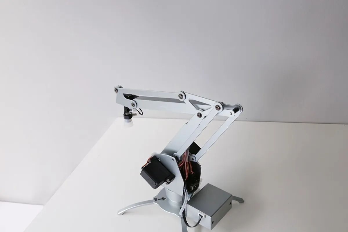
To draw a C-space obstacle, you check each grid cell: put the arm in that pose and ask, “Does any link touch the obstacle?” If yes, colour the cell. A small bottle on the table can become a large, oddly-shaped blob in C-space, because many different angle pairs swing a link through it. If the upper arm itself passes through the obstacle at some shoulder angle, then every elbow angle at that shoulder angle is blocked — a full stripe on the map.
Visual
Visualise it: explore a 2-joint configuration space
Move the arm and watch the **dot** move on the C-space map. Every arm shape is one dot. Find the regions where the arm hits something — they show up as **forbidden areas** on the map.
Interactive · Configuration space explorer · Educational 2R


Educational C-space sketch for planar 2R — not OMPL / not MoveIt / not 6DOF C-space.
Code lab
Code lab: draw a 2R arm’s C-space in text
This script sweeps θ₁ and θ₂ from −180° to 180° in 15° steps (25 × 25 = 625 cells). For each cell it checks joint limits (shoulder 0°–180°, elbow −150°–150°), then checks whether either link touches a circular obstacle at (0.10, 0.10) m with radius 0.03 m. x = outside limits, # = collision, . = free. Run it with python3 cspace_grid.py.
"""cspace_grid.py - draw the configuration space (C-space) of a planar 2R arm.
Each cell is one (theta1, theta2) pair. '#' = arm hits the obstacle, 'x' = outside joint limits, '.' = free."""
import math

L1, L2 = 0.12, 0.10              # link lengths in metres (hobby-arm scale)
OBST = (0.10, 0.10, 0.03)        # obstacle circle: centre x, y and radius (m)
LIMIT1 = (0, 180)                # shoulder limits (deg)
LIMIT2 = (-150, 150)             # elbow limits (deg)
STEP = 15

def seg_hits_circle(p, q, c, r):
    (px, py), (qx, qy), (cx, cy) = p, q, c
    dx, dy = qx - px, qy - py
    t = max(0.0, min(1.0, ((cx - px) * dx + (cy - py) * dy) / (dx * dx + dy * dy)))
    nx, ny = px + t * dx, py + t * dy
    return math.hypot(cx - nx, cy - ny) <= r

def arm_points(t1, t2):
    a, b = math.radians(t1), math.radians(t1 + t2)
    elbow = (L1 * math.cos(a), L1 * math.sin(a))
    tip = (elbow[0] + L2 * math.cos(b), elbow[1] + L2 * math.sin(b))
    return (0.0, 0.0), elbow, tip

t1s = list(range(-180, 181, STEP))
t2s = list(range(-180, 181, STEP))
free = blocked = limited = 0
print("theta2 (rows, deg) vs theta1 (columns, -180..180 step 15)")
for t2 in reversed(t2s):
    row = ""
    for t1 in t1s:
        if not (LIMIT1[0] <= t1 <= LIMIT1[1] and LIMIT2[0] <= t2 <= LIMIT2[1]):
            row += "x"; limited += 1; continue
        base, elbow, tip = arm_points(t1, t2)
        hit = seg_hits_circle(base, elbow, OBST[:2], OBST[2]) or seg_hits_circle(elbow, tip, OBST[:2], OBST[2])
        row += "#" if hit else "."
        blocked += hit; free += not hit
    print(f"{t2:5d} {row}")
total = free + blocked + limited
print(f"\ncells: {total}  free: {free}  obstacle: {blocked}  outside limits: {limited}")
for pose in [(45, 0), (90, -90), (30, 60)]:
    _, _, tip = arm_points(*pose)
    print(f"pose (theta1, theta2) = {pose} -> tip at x={tip[0]:.3f} m, y={tip[1]:.3f} m")
Output (run with python3 cspace_grid.py)
theta2 (rows, deg) vs theta1 (columns, -180..180 step 15)
  180 xxxxxxxxxxxxxxxxxxxxxxxxx
  165 xxxxxxxxxxxxxxxxxxxxxxxxx
  150 xxxxxxxxxxxx...#.........
  135 xxxxxxxxxxxx...#.........
  120 xxxxxxxxxxxx...#.........
  105 xxxxxxxxxxxx####.........
   90 xxxxxxxxxxxx####.........
   75 xxxxxxxxxxxx.###.........
   60 xxxxxxxxxxxx..##.........
   45 xxxxxxxxxxxx..##.........
   30 xxxxxxxxxxxx..##.........
   15 xxxxxxxxxxxx...#.........
    0 xxxxxxxxxxxx...#.........
  -15 xxxxxxxxxxxx...#.........
  -30 xxxxxxxxxxxx...##........
  -45 xxxxxxxxxxxx...##........
  -60 xxxxxxxxxxxx...##........
  -75 xxxxxxxxxxxx...###.......
  -90 xxxxxxxxxxxx...####......
 -105 xxxxxxxxxxxx...####......
 -120 xxxxxxxxxxxx...#.........
 -135 xxxxxxxxxxxx...#.........
 -150 xxxxxxxxxxxx...#.........
 -165 xxxxxxxxxxxxxxxxxxxxxxxxx
 -180 xxxxxxxxxxxxxxxxxxxxxxxxx

cells: 625  free: 230  obstacle: 43  outside limits: 352
pose (theta1, theta2) = (45, 0) -> tip at x=0.156 m, y=0.156 m
pose (theta1, theta2) = (90, -90) -> tip at x=0.100 m, y=0.120 m
pose (theta1, theta2) = (30, 60) -> tip at x=0.104 m, y=0.160 mReal world
Configuration space in real robots
- Motion planners (in Stage 9 and 13 and in tools like MoveIt) search the free C-space for a path, then send joint trajectories to the robot.
- Joint limits in every industrial controller cut the C-space down to a box — the robot simply refuses commands outside it.
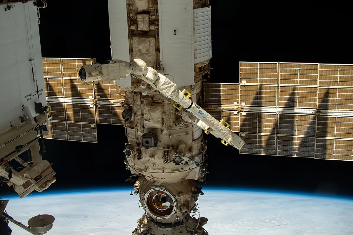
- Space robotics: arms on the ISS, like the European Robotic Arm, work close to station modules, so knowing which configurations collide matters enormously.
- Your 6DOF arm: each servo’s soft limits (Lesson 13) define its C-space box; the table and the base itself are C-space obstacles.
Bench build
Bench build: a paper C-space for your cardboard arm
Use the cardboard 2R arm from Lesson 3 and a cup or bottle as the obstacle. You will build the C-space map by hand — the best way to really understand it.
Make a protractor base
Draw a protractor (0°–180°) around the shoulder pin on the table, and a small one at the elbow on the upper-arm strip.
Draw the grid
On graph paper, make a 7 × 9 grid: θ₁ = 0, 30, …, 180 across and θ₂ = −120, −90, …, 120 up.
Test each cell
Set the arm to each pair. If any part touches the cup, colour the cell red. If a joint can’t reach the angle, shade it grey.
Plan a path
Mark a start pose and a goal pose on opposite sides of the red blob. Draw a path through white cells only.
Test the path
Move the cardboard arm along your path, cell by cell. Does it miss the cup? If not, your grid was too coarse — add cells near the blob.
Debugging
Debugging your C-space map
| Problem | Why it happens | Fix |
|---|---|---|
| Path looks free on the map but the arm hits | Grid too coarse — the collision is between cells | Use smaller steps near obstacles; add a safety margin to the obstacle radius |
| Map looks mirrored | θ₂ measured the opposite way, or axes swapped | Write the sign convention on the map; check one pose by hand |
| Too many blocked cells | Obstacle radius or link width too big | Measure again; links have width — model it honestly |
| Arm moves through a forbidden band | Joint limits not enforced in code | Clamp every command to its limits (Lesson 13) |
| Script is slow | Too many cells (6 joints × fine steps explodes) | That is why real planners sample C-space instead of gridding it |
Think
Think about it
Think
Meera says: “My arm’s tip can reach the point (0.10, 0.12) m, so I just send that point and it’s done.” Arjun says: “Which way should the elbow bend?” Using C-space, explain why both of them are partly right, and why it matters if there is a bottle near the elbow.
Experiment
Try it in the lab: draw your own C-space map
Thirty minutes with the C-space explorer, the script and your paper map. You will see one obstacle from two points of view — table and angle map.
Experiment
Draw your own C-space map
You will need
- Configuration space explorer (below, runs in your browser)
- Graph paper, coloured pencils
- Cardboard 2R arm from Lesson 3, a plastic cup
- Optional: `cspace_grid.py`
Steps
- In the explorer, move the arm until it touches the obstacle. Note the joint angles. Find two more touching poses.
- Run `cspace_grid.py`. Find the three poses printed at the bottom on the map grid (round to the nearest 15°). Are they free?
- Build your paper map with the cardboard arm and cup (bench section).
- Plan a path from (0°, 0°) to (150°, 0°) through free cells. Write the sequence of cells.
- Move the obstacle in the script to match your cup’s real position and compare the script’s map with your paper map.
Interactive · Configuration space explorer · Educational 2R
Educational C-space sketch for planar 2R — not OMPL / not MoveIt / not 6DOF C-space.
A small object in the room becomes a large, strangely shaped forbidden region in C-space. Paths that look straight in the room can be curved in C-space, and vice versa.
Knowledge check
Check your understanding
Knowledge check
1. A robot’s configuration is…
2. The dimension of a robot’s C-space equals…
3. For a 2R arm, one point in C-space is…
4. Without joint limits, the C-space of a 2R arm has the shape of…
5. In `cspace_grid.py`, why is there a full vertical stripe of `#` at θ₁ = 45°?
6. Free C-space means configurations that are…
7. Why can two different C-space points give the same tip position?
8. A path looks free on your coarse grid but the arm hits the cup. The best fix is…
9. Why don’t planners grid the C-space of a 6R arm?
Mini assignment
Hands-on assignment
Mini assignment
Map the angle-land of your arm
Draw the C-space of your cardboard (or real) 2R arm with joint limits and one obstacle, plan a safe path on it, and test the path for real.
Deliverables
- A coloured C-space map (paper or script output) with limits, the obstacle region, a start, a goal and a planned path.
- A photo or short video of the cardboard arm following the path without touching the obstacle.
- Your edited `cspace_grid.py` with your own link lengths and obstacle position, and its output.
- Three sentences explaining the difference between C-space and workspace, using your own map as the example.
Do this, step by step
- Measure your cardboard (or real) 2R arm: both link lengths and the joint limits of each joint.
- Set those numbers and one obstacle position in
cspace_grid.py, run it and look at the blocked region in the θ1–θ2 grid. - Colour the map on paper: limits, obstacle blob, a start, a goal, and a path between them that stays in free space.
- Move the real arm along your path, joint by joint, and record a photo or short video showing it never touches the obstacle.
- Write three sentences explaining C-space vs workspace using your own map as the example.
Stuck? Hints, one at a time
- Hint 1: Measure your link lengths from pin to pin, in metres, and put them in
L1,L2. - Hint 2: Measure the cup’s centre (x, y) from the shoulder pin, with x along the table edge and y away from you.
- Hint 3: If the map has no
#cells, the obstacle is out of reach — move it closer than L₁ + L₂. - Hint 4: For the path, move one joint at a time first (straight lines on the map). Diagonal moves come later.
Challenges (pick by level)
- 🟢 Easy: Compute the tip position for (θ₁, θ₂) = (0°, 90°) by hand with L₁ = 0.12, L₂ = 0.10. Check it with the formula in the script.
- 🟢 Easy: Shade the joint-limit bands on a blank 2-D map for shoulder 0°–180° and elbow −150°–150°.
- 🟡 Medium: Add a second obstacle to the script. Is there still a free path from θ₁ = 0° to θ₁ = 180°?
- 🟡 Medium: Make the script print the free-cell percentage. How does it change if the obstacle radius doubles?
- 🟠 Hard-ish: Add a breadth-first search over free cells to find a path from a start cell to a goal cell automatically. *Hint:* neighbours are the four cells up/down/left/right.
- 🔴 Hard: Model links as thick bars (add half the link width to the obstacle radius) and compare maps.
- ⚫ Expert: Read Modern Robotics Section 10.2.1 on C-space obstacles and write a one-page explanation, with your own figure, of how a round obstacle maps into a 2R arm’s C-space.
Next step
You can describe *where* a robot can be. In Lesson 5 — Actuators & Transmissions you find out *what moves it there*: motors, gears, belts and screws — and how to size them so a joint can actually hold its load.
Look back: Lesson 3: Joints, Links & DOF. Next: Lesson 5: Actuators & Transmissions. Related: Stage 9 — Trajectory Planning and Stage 13 — Perception, Planning & Manipulation.
Sources
- Modern Robotics — K. M. Lynch & F. C. Park (preprint PDF) — Ch. 2: configuration and C-space definitions; dimension equals DOF; C-space of a 2R arm is a torus T²; with joint limits it becomes a product of closed intervals; free C-space; Ch. 10.2.1: configuration space obstacles.
- Photos: Wikimedia Commons (credits under each image).
Self-attested for now — keep artifacts in your lab notebook.
Complete
Today's goal
0 of 1 done today
Mark this lesson complete when you have worked the experiment, knowledge check, and assignment (even roughly).