
Kinematics & Inverse Kinematics · Lesson 13
Analytical vs Numerical IK
Est. 60–80 min
Why
Why this lesson matters
In Lesson 12 you solved IK with a formula (law of cosines). That is analytical (closed-form) IK: fast, exact and it gives *every* answer — but a formula only exists for some arm shapes. Numerical IK works for almost any arm you can write FK for: it starts from a guess and repeatedly nudges the joints towards the target using the Jacobian. It is general, but it needs a good starting guess, returns one answer, and can fail.
By the end of this lesson you will be able to: compare analytical and numerical IK on speed, answers, generality and failure modes; explain the Newton–Raphson IK step θ ← θ + J†·e; build a position Jacobian for a planar arm; see how the starting guess picks the answer; handle unreachable targets with damped least squares; and solve a redundant 3-link arm on an Arduino.
Concept
Two ways to solve IK
Side by side
| Analytical (closed-form) | Numerical (iterative) | |
|---|---|---|
| Idea | Geometry/algebra gives a formula for each joint | Start from a guess, step towards the target, repeat |
| Answers | All of them (e.g. both elbows) | One — usually the one nearest the starting guess |
| Speed | Very fast, fixed time | Slower; number of steps varies |
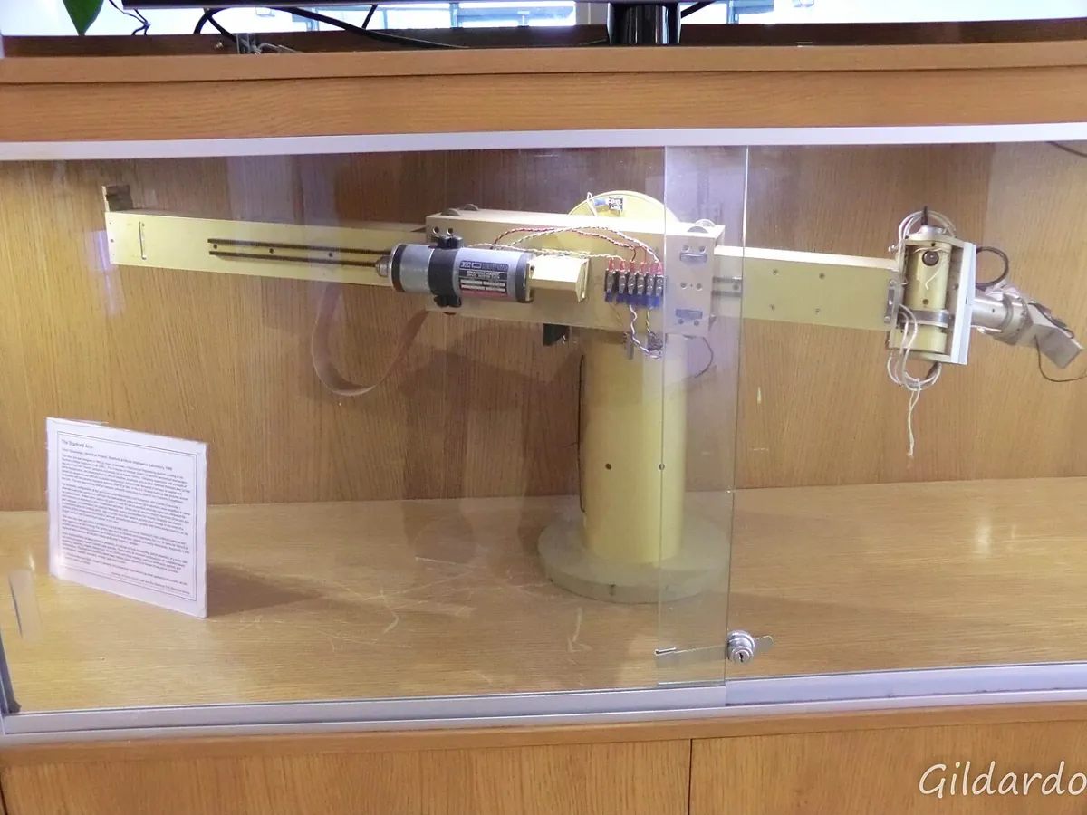
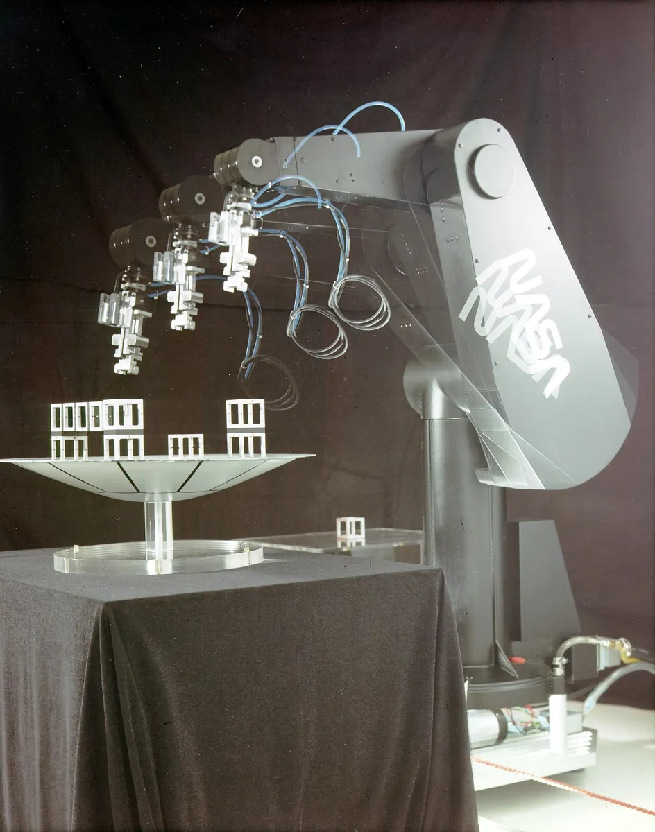
| Works for | Specific shapes (2R, many 6-axis arms with a spherical wrist, PUMA, Stanford Arm) | Almost any chain with FK and a Jacobian, including redundant arms |
| Fails when | No formula exists for that shape | Bad guess, near a singularity, unreachable target |
| Typical use | Industrial controllers for standard arms | Odd shapes, extra joints, extra goals, animation |
The Newton–Raphson IK step
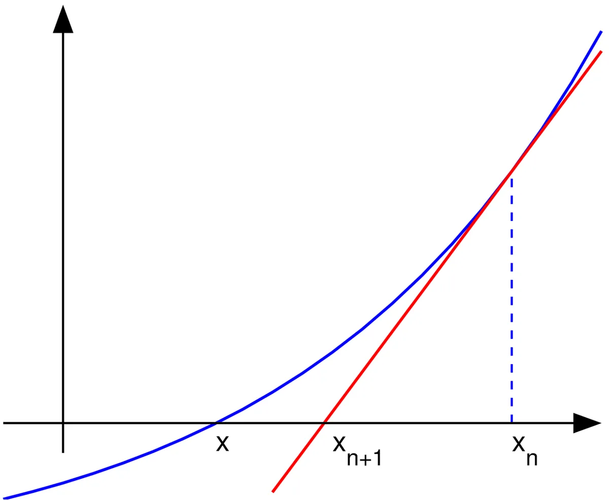
The Jacobian J says how much the tip moves when each joint turns a tiny bit. If the tip is off by an error e = target − FK(θ), then a joint change Δθ with J·Δθ ≈ e should fix it. So:
θ = starting guess
repeat:
    e  = target − FK(θ)            # how far off are we?
    if |e| < tolerance: done
    θ  = θ + J†(θ) · e               # J† = pseudoinverse of the Jacobian

Damped version (more stable near trouble):
Δθ = Jᵀ (J Jᵀ + λ² I)⁻¹ · eVisual
Visualise it: the closed-form 2R solver
The lab’s solver is analytical: law of cosines for a 2R arm, both elbow answers at once, each verified by FK. Educational and simplified — not full 6DOF IK.
Interactive · IK solver lab (analytical 2R — educational)


Workflow: target → IK → joints → FK verify → residual. Not a black box — elbow-up/down closed form. Not full 6DOF analytic IK.
Status · ok
2 analytical solution(s) (2R planar).
θ₁
-12.2°
θ₂
92.3°
FK err
0.000
Code lab
Code lab: ik_numeric.py
ik_numeric.py builds the position Jacobian of a planar arm, takes pseudoinverse (and damped) steps, and compares the result with the closed-form 2R answers. It also times both on your computer, tries an unreachable target, and solves a redundant 3-link arm from three different starting guesses.
# ik_numeric.py - analytical vs numerical inverse kinematics on planar arms.
# Analytical: a formula (law of cosines) - instant, gives ALL answers, but only exists for some arms.
# Numerical: Newton-Raphson with the Jacobian (Modern Robotics 6.2) - works for any chain you can
# write FK for, but needs a starting guess, iterates, and returns ONE answer (near the guess).
import math
import time

L = [10.0, 8.0]                       # 2R link lengths, cm


def fk(q, links):
    x = y = a = 0.0
    for qi, li in zip(q, links):
        a += qi
        x += li * math.cos(a)
        y += li * math.sin(a)
    return x, y


def jacobian(q, links):
    """2 x n position Jacobian: how the tip (x, y) moves per radian of each joint."""
    J = [[0.0] * len(q) for _ in range(2)]
    for i in range(len(q)):
        a = sum(q[:i])
        for k in range(i, len(q)):
            a += q[k]
            J[0][i] += -links[k] * math.sin(a)
            J[1][i] += links[k] * math.cos(a)
    return J


def pinv_step(J, e, damping=0.0):
    """dq = J^T (J J^T + lambda^2 I)^-1 e  (pseudoinverse; damped if lambda > 0)."""
    a = sum(J[0][i] * J[0][i] for i in range(len(J[0]))) + damping ** 2
    b = sum(J[0][i] * J[1][i] for i in range(len(J[0])))
    d = sum(J[1][i] * J[1][i] for i in range(len(J[0]))) + damping ** 2
    det = a * d - b * b
    if abs(det) < 1e-12:
        return None
    w0 = (d * e[0] - b * e[1]) / det
    w1 = (-b * e[0] + a * e[1]) / det
    return [J[0][i] * w0 + J[1][i] * w1 for i in range(len(J[0]))]


def ik_numeric(target, q0, links, tol=1e-6, max_iter=100, damping=0.0):
    q = list(q0)
    for it in range(max_iter + 1):
        x, y = fk(q, links)
        e = (target[0] - x, target[1] - y)
        if math.hypot(*e) < tol:
            return q, it, math.hypot(*e)
        if it == max_iter:
            break
        dq = pinv_step(jacobian(q, links), e, damping)
        if dq is None:
            break
        q = [qi + dqi for qi, dqi in zip(q, dq)]
    x, y = fk(q, links)
    return q, it, math.hypot(target[0] - x, target[1] - y)


def ik_analytic(target, l1, l2):
    x, y = target
    d2 = x * x + y * y
    c = (d2 - l1 * l1 - l2 * l2) / (2 * l1 * l2)
    if abs(c) > 1:
        return []
    return [(math.atan2(y, x) - math.atan2(l2 * math.sin(s * math.acos(c)), l1 + l2 * math.cos(s * math.acos(c))),
             s * math.acos(c)) for s in (1, -1)]


deg = lambda q: "(" + ", ".join(f"{round(math.degrees(v), 2) + 0.0:7.2f}" for v in q) + ")"
T = (12.0, 6.0)

print(f"1) 2R arm {L}, target {T}")
for q in ik_analytic(T, *L):
    print(f"   analytical      q = {deg(q)}  error {math.dist(fk(q, L), T):.1e} cm")
for guess in ((0.0, 0.5), (1.5, -0.5), (0.0, 0.0)):
    q, it, err = ik_numeric(T, guess, L)
    note = "  <- STUCK: arm stretched straight, Jacobian singular (Lesson 14)" if err > 1e-3 else ""
    print(f"   numerical from {deg(guess)}: q = {deg(q)}  in {it:3d} iterations, error {err:.1e} cm{note}")

t0 = time.perf_counter()
for _ in range(2000):
    ik_analytic(T, *L)
t1 = time.perf_counter()
for _ in range(2000):
    ik_numeric(T, (0.0, 0.5), L)
t2 = time.perf_counter()
print(f"   time per solve on this computer: analytical {1e6 * (t1 - t0) / 2000:.1f} us, numerical {1e6 * (t2 - t1) / 2000:.1f} us"
      " (varies by machine)")

print("\n2) Target out of reach (25, 0): analytical says no answer; numerical never reaches tol")
print(f"   analytical answers: {ik_analytic((25.0, 0.0), *L)}")
for lam, label in ((0.0, "plain   "), (4.0, "damped  ")):
    q, it, err = ik_numeric((25.0, 0.0), (0.3, 0.3), L, max_iter=50, damping=lam)
    tip = tuple(round(v, 2) + 0.0 for v in fk(q, L))
    print(f"   {label} lambda={lam}: after {it} it q = {deg(q)}, tip {tip}, still {err:.2f} cm away")
print("   -> plain Newton-Raphson can wander; damped least squares stretches towards the target")
print("      (the closest it can get). Either way: ALWAYS check the final error before moving.")

L3 = [10.0, 8.0, 5.0]
print(f"\n3) Redundant 3R arm {L3}, target {T} (position only: 3 joints, 2 numbers -> infinitely many answers)")
for guess in ((0.0, 0.5, 0.5), (1.0, -1.0, -0.5), (-0.5, 1.0, 1.0)):
    q, it, err = ik_numeric(T, guess, L3)
    print(f"   from {deg(guess)} -> q = {deg(q)}  in {it:2d} it, error {err:.1e} cm")
print("   -> every answer reaches the same point; the guess decides which one you get")
Output (run with python3 ik_numeric.py; timings vary by machine)
1) 2R arm [10.0, 8.0], target (12.0, 6.0)
   analytical      q = (  -9.83,   84.26)  error 0.0e+00 cm
   analytical      q = (  62.96,  -84.26)  error 8.9e-16 cm
   numerical from (   0.00,   28.65): q = (  -9.83,   84.26)  in   5 iterations, error 5.8e-09 cm
   numerical from (  85.94,  -28.65): q = (  62.96,  -84.26)  in   6 iterations, error 1.3e-07 cm
   numerical from (   0.00,    0.00): q = (   0.00,    0.00)  in   0 iterations, error 8.5e+00 cm  <- STUCK: arm stretched straight, Jacobian singular (Lesson 14)
   time per solve on this computer: analytical 1.5 us, numerical 28.9 us (varies by machine)

2) Target out of reach (25, 0): analytical says no answer; numerical never reaches tol
   analytical answers: []
   plain    lambda=0.0: after 50 it q = (6108.55, -4989.62), tip (16.02, 3.04), still 9.48 cm away
   damped   lambda=4.0: after 50 it q = (   0.00,    0.00), tip (18.0, 0.0), still 7.00 cm away
   -> plain Newton-Raphson can wander; damped least squares stretches towards the target
      (the closest it can get). Either way: ALWAYS check the final error before moving.

3) Redundant 3R arm [10.0, 8.0, 5.0], target (12.0, 6.0) (position only: 3 joints, 2 numbers -> infinitely many answers)
   from (   0.00,   28.65,   28.65) -> q = ( -26.13,   74.37,   69.23)  in  5 it, error 1.1e-12 cm
   from (  57.30,  -57.30,  -28.65) -> q = (  85.24,  -85.96,  -49.92)  in  4 it, error 9.2e-10 cm
   from ( -28.65,   57.30,   57.30) -> q = ( -26.31,   74.70,   68.70)  in  4 it, error 1.7e-10 cm
-> every answer reaches the same point; the guess decides which one you getTry it: this lab uses the analytical (closed-form) 2R solver. Notice it shows both elbow answers instantly — the thing a numerical solver cannot do in one run. (Educational, simplified.)
Interactive · IK solver lab (analytical 2R — educational)
Workflow: target → IK → joints → FK verify → residual. Not a black box — elbow-up/down closed form. Not full 6DOF analytic IK.
Status · ok
2 analytical solution(s) (2R planar).
θ₁
-12.2°
θ₂
92.3°
FK err
0.000
Simulator
Try it in the simulator
Simulator · Kinematics
2-link planar arm: forward & inverse kinematics
Move the joints (FK) or drag the target (IK) and compare the elbow-up and elbow-down solutions.
Loading simulator…
Formulas used
- x = L1·cos θ1 + L2·cos(θ1 + θ2)
- y = L1·sin θ1 + L2·sin(θ1 + θ2)
- cos θ2 = (x² + y² − L1² − L2²) / (2·L1·L2)
- θ1 = atan2(y, x) − atan2(L2·sin θ2, L1 + L2·cos θ2)
Model & limits
Ideal rigid links, point joints, no joint limits or collisions. Reachable only when |L1 − L2| ≤ r ≤ L1 + L2.
Real world
Both methods in the real world
- Standard industrial arms: many 6-axis arms have a spherical wrist, which allows the problem to be split and solved in closed form (PUMA-type and Stanford-type arms are classic examples in *Modern Robotics*).
- Polishing real arms: analytical answers can be used as the starting guess for a numerical solver that accounts for small real-world imperfections.
- Animation and odd shapes: computer animation tools often use Newton’s method for IK, because characters have many joints and no neat formula.
- Redundant arms: arms with 7 or more joints have infinitely many answers for a pose; numerical methods choose one that also meets extra goals.
Bench build
Bench build: numerical IK on an Arduino, 3-servo arm
Add a third link (5 cm) to the Lesson 12 two-servo arm. With three joints and only (x, y) to hit, the arm is redundant — a perfect job for numerical IK. ik_numeric_3servo.ino runs damped least-squares steps on the Arduino, starting from the arm’s current pose so it moves to a nearby answer, prints iterations, error and solve time, and refuses to move if it failed.
Power
Three servos on their own 5–6 V supply rated 3 A or more, supply GND joined to Arduino GND. Signals on pins 5, 6 and 9.
Zero
Set ZERO[] so each link points straight along the previous one at 0°.
Test
Type 12 6, then 14 3, then 12 6 again. Does the arm return to the same pose? (Warm start says it should be close.)
Break it
Type 30 0 (out of reach). The sketch should print a big error and refuse to move.
// ik_numeric_3servo.ino - NUMERICAL IK running on the Arduino for a 3-servo planar arm
// (shoulder, elbow, wrist in one vertical or flat plane). Three joints, two target numbers (x, y):
// the arm is redundant, so there is no single formula - we iterate with the Jacobian instead,
// starting from the CURRENT pose so the arm moves to the nearest answer (Modern Robotics 6.2).
// Type a target "x y" in cm. The sketch iterates (damped least squares), prints iterations,
// final error and solve time, refuses if the error stays above 0.2 cm or a joint leaves -80..80,
// and then moves all three servos slowly together.
// SERVOS run from their OWN 5-6 V supply (3 A or more for three servos), NEVER from the
// Arduino 5 V pin. Join the supply GND to Arduino GND. Signals: pins 5, 6, 9.
#include <Servo.h>
const float LEN[3] = {10.0, 8.0, 5.0};             // cm - MEASURE
const int ZERO[3] = {90, 90, 90};                  // servo command for 0 deg
const int PINS[3] = {5, 6, 9};
const float QMAX = radians(80);
const float LAMBDA = 0.5;                          // damping: bigger = calmer but slower
Servo s[3];
float q[3] = {0.3, 0.5, 0.5};                      // current joint angles, radians

void fk(const float *qq, float &x, float &y) {
  float a = 0; x = 0; y = 0;
  for (int i = 0; i < 3; i++) { a += qq[i]; x += LEN[i] * cos(a); y += LEN[i] * sin(a); }
}

// one damped least-squares step: dq = J^T (J J^T + lambda^2 I)^-1 e
void step(float *qq, float ex, float ey) {
  float J[2][3];
  for (int i = 0; i < 3; i++) {
    J[0][i] = 0; J[1][i] = 0;
    float a = 0;
    for (int k = 0; k < i; k++) a += qq[k];
    for (int k = i; k < 3; k++) { a += qq[k]; J[0][i] -= LEN[k] * sin(a); J[1][i] += LEN[k] * cos(a); }
  }
  float A = LAMBDA * LAMBDA, B = 0, D = LAMBDA * LAMBDA;
  for (int i = 0; i < 3; i++) { A += J[0][i] * J[0][i]; B += J[0][i] * J[1][i]; D += J[1][i] * J[1][i]; }
  float det = A * D - B * B;
  float w0 = (D * ex - B * ey) / det, w1 = (-B * ex + A * ey) / det;
  for (int i = 0; i < 3; i++) qq[i] += J[0][i] * w0 + J[1][i] * w1;
}

void writeServos(const float *qq) {
  for (int i = 0; i < 3; i++) s[i].write(ZERO[i] + (int)round(degrees(qq[i])));
}

void setup() {
  for (int i = 0; i < 3; i++) s[i].attach(PINS[i]);
  writeServos(q);
  Serial.begin(115200);
  Serial.println(F("Type target: x y  (cm)"));
}

void loop() {
  if (!Serial.available()) return;
  float tx = Serial.parseFloat(), ty = Serial.parseFloat();
  while (Serial.available()) Serial.read();
  float g[3] = {q[0], q[1], q[2]};                 // warm start from the current pose
  unsigned long t0 = micros();
  int it = 0;
  float x, y, err = 1e9;
  for (; it < 60; it++) {
    fk(g, x, y);
    err = sqrt(sq(tx - x) + sq(ty - y));
    if (err < 0.05) break;
    step(g, tx - x, ty - y);
  }
  unsigned long dt = micros() - t0;
  Serial.print(F("iterations ")); Serial.print(it); Serial.print(F("  error "));
  Serial.print(err, 3); Serial.print(F(" cm  time ")); Serial.print(dt); Serial.println(F(" us"));
  for (int i = 0; i < 3; i++)
    if (fabs(g[i]) > QMAX) { Serial.println(F("Joint limit exceeded - not moving.")); return; }
  if (err > 0.2) { Serial.println(F("Could not reach target - not moving.")); return; }
  float from[3] = {q[0], q[1], q[2]};              // move slowly: 40 small steps
  for (int k = 1; k <= 40; k++) {
    float m[3];
    for (int i = 0; i < 3; i++) m[i] = from[i] + (g[i] - from[i]) * k / 40.0;
    writeServos(m);
    delay(20);
  }
  for (int i = 0; i < 3; i++) q[i] = g[i];
}
Debugging
Debugging numerical IK
| Symptom | Likely cause | Fix |
|---|---|---|
| Solver stops at once with a big error | Starting guess at a singularity (arm straight) | Start from a slightly bent pose |
| Angles grow to hundreds of degrees | Target unreachable, no damping | Check reach first; use damping λ; wrap angles |
| Arm flips to a far-away pose | Started from a fixed guess instead of the current pose | Warm-start from the current joint angles |
| Converges very slowly | Damping too large | Reduce λ (or reduce it as the error shrinks) |
| Converges to the wrong point | Jacobian sign error | Check J numerically: nudge one joint, compare tip change |
| Arduino answer differs slightly from Python | float (32-bit) vs Python’s 64-bit numbers | Accept small differences; use a tolerance like 0.05 cm |
Think
Think about it
Think
Zoya says, “Numerical IK works for every arm, so nobody should bother with formulas.” Give two reasons why industrial controllers still love analytical IK.
Experiment
Try it in the lab
About 45 minutes with ik_numeric.py, and optionally the 3-servo arm.
Experiment
Race the two methods
You will need
- `ik_numeric.py` and Python 3
- Optional: 3-servo planar arm, separate 5–6 V servo supply (3 A+), Arduino UNO
Steps
- Run `ik_numeric.py` and note iterations and solve times.
- Find a starting guess that makes Newton–Raphson land on the *other* elbow answer for (12, 6).
- Start from (5°, 5°) instead of (0°, 0°). Does it escape the stretched-arm trap?
- For the out-of-reach target, try λ = 1 and λ = 2. Which one ends closest to (18, 0)?
- For the 3R arm, add a fourth starting guess and compare the answer with the other three.
- If you built the 3-servo arm, record iterations and solve time printed by the Arduino.
Interactive · IK solver lab (analytical 2R — educational)
Workflow: target → IK → joints → FK verify → residual. Not a black box — elbow-up/down closed form. Not full 6DOF analytic IK.
Status · ok
2 analytical solution(s) (2R planar).
θ₁
-12.2°
θ₂
92.3°
FK err
0.000
Formulas are instant and complete but need a special arm shape. Iteration is general but depends on the starting guess, can get stuck at singularities, and always needs an error check. Warm-starting from the current pose keeps motion smooth and predictable.
Knowledge check
Check your understanding
Knowledge check
1. Analytical IK means…
2. A numerical IK solver usually returns…
3. In the Newton–Raphson IK step θ ← θ + J†·e, what is e?
4. Why did the solver get stuck starting from (0°, 0°)?
5. What does damping (λ) do in damped least squares?
6. A redundant 3R planar arm reaching only (x, y) has…
7. A good way to combine both methods is…
Mini assignment
Hands-on assignment
Mini assignment
Method choice report
Write a one-page report recommending analytical or numerical IK for three robots.
Deliverables
- Robot A: your Stage 6 arm (pick from above). Robot B: a 3-link planar drawing arm. Robot C: a 7-joint arm.
- For each: which method, why, and what could go wrong.
- Your measured iterations and timings from `ik_numeric.py` (and the Arduino, if built).
- A starting guess that makes Newton–Raphson fail for (12, 6), and why it fails.
- Your rule for rejecting a numerical answer (error and limits).
Do this, step by step
- Run
python3 ik_numeric.pyand note the iterations and the time per solve on your computer (it will differ from the printed output). - Change the starting guess for (12, 6) until Newton–Raphson fails or gives the other elbow family. Write down the guess and why.
- Change the tolerance from 1e-6 to 1e-3 and count how many iterations you save.
- Write your rule for accepting a numerical answer: tip error below a limit and every joint within its limits.
- Fill in the report for robots A, B and C: analytical or numerical, why, and what could go wrong.
Stuck? Hints, one at a time
- Newton–Raphson follows the slope (Jacobian) from the start guess, so a guess near the other elbow family finds that one.
- A stretched-out start (q2 = 0) makes J nearly singular, so steps get huge or the solver stalls; damping helps.
- Always run FK on the final answer and check the error yourself.
Challenges (pick by level)
- 🟢 Easy: Change the tolerance to 1e-3 and count how many iterations you save.
- 🟢 Easy: Explain in your own words what one column of the Jacobian means.
- 🟡 Medium: Check the Jacobian numerically: nudge each joint by 0.001 rad and compare the tip change with J.
- 🟠 Hard-ish: Add a wrist-angle goal to the 3R solver (x, y and φ = q1 + q2 + q3) — now it is no longer redundant.
- 🔴 Hard: Implement Cyclic Coordinate Descent (CCD) and compare its iterations with Newton–Raphson.
- ⚫ Research: Read *Modern Robotics* Section 6.2 and summarise how the method changes when you want a full pose (with the body Jacobian).
Next step
You met two kinds of trouble: several valid answers, and a stretched arm where the solver got stuck. In Lesson 14 — Multiple Solutions & Singularities you will learn to choose between answers and to recognise and avoid singular poses.
Look back: Lesson 12: Inverse Kinematics — Concept. Next: Lesson 14: Multiple Solutions & Singularities. Related: Stage 1: Matrices and Stage 14 — Advanced Robotics / RL.
Sources
- Modern Robotics — K. M. Lynch & F. C. Park (book home page, free preprint) — Chapter 6: analytic IK (PUMA and Stanford-type arms), 6.2 Numerical IK with Newton–Raphson and the pseudoinverse, initial guess near a solution, analytical answers as initial guesses.
- Wikipedia — Inverse kinematics — analytical vs numerical approaches; animation tools often use Newton’s method.
- Wikipedia — Newton’s method — the tangent-line iteration behind Newton–Raphson.
- Stanford Arm description from its Wikimedia Commons file page (credit under the photo).
- Photos: Wikimedia Commons (credits under each image).
Self-attested for now — keep artifacts in your lab notebook.
Complete
Today's goal
0 of 1 done today
Mark this lesson complete when you have worked the experiment, knowledge check, and assignment (even roughly).